1. Introduction

• Proofs are treated as first class objects: they can be normalized and then used for reading off an instance if the proven formula is existential, or changed for program development by proof transformation.
• To keep control over the complexity of extracted programs, we follow Kreisel’s proposal and aim at a theory with a strong language and weak existence axioms. It should be conservative over (a fragment of) arithmetic.
• Minlog is based on minimal rather than classical or intuitionistic logic. This more general setting makes it possible to implement program extraction from classical proofs, via a refined A-translation (cf. [3]).
• Constants are intended to denote computable functionals. Since their (mathematically correct) domains are the Scott-Ershov partial continuous functionals, this is the intended range of the quantifiers.
• Variables carry (simple) types, with free algebras as base types. The latter need not be finitary (so we allow e.g. countably branching trees), and can be simultaneously generated. Type parameters (ML style) are allowed, but we keep the theory predicative and disallow type quantification.
• To simplify equational reasoning, the system identifies terms with the same normal form. A rich collection of rewrite rules is provided, which can be extended by the user. Decidable predicates are implemented via boolean valued functions, hence the rewrite mechanism applies to them as well.

We now describe in more details some of these features.

1.1. Simultaneous free algebras. A free algebra is given by constructors, for instance zero and successor for the natural numbers. We want to treat other data types as well, like lists and binary trees. When dealing with inductively defined sets, it will also be useful to explicitely refer to the generation tree. Such trees are quite often countably branching, and hence we allow infinitary free algebras from the outset.

The freeness of the constructors is expressed by requiring that their ranges are disjoint and that they are injective. Moreover, we view the free algebra as a domain and require that its bottom element is not in the range of the constructors. Hence the constructors are total and non-strict. For the notion of totality cf. [12, Chapter 8.3].

In our intended semantics we do not require that every semantic object is the denotation of a closed term, not even for finitary algebras. One reason is that for normalization by evaluation (cf. [4]) we want to allow term families in our semantics.

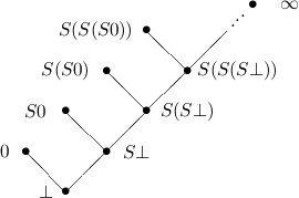
To make a free algebra into a domain and still have the constructors injective and with disjoint ranges, we model e.g. the natural numbers as shown in Figure 1.

Notice that for more complex algebras we usually need many more “infinite” elements; this is a consequence of the closure of domains under suprema. To make dealing with such complex structures less annoying, we will normally restrict attention to the total elements of a domain, in this case – as expected – the elements labelled 0, S0, S(S0) etc.

1.2. Partial continuous functionals. As already mentioned, the (mathematically correct) domains of computable functionals have been identified by Scott and Ershov as the partial continuous functionals; cf. [12]. Since we want to deal with computable functionals in our theory, we consider it as mandatory to accommodate their domains. This is also true if one is interested in total functionals only; they have to be treated as particular partial continuous functionals. We will make use of predicate constants Total_ρ with the total functionals of type ρ as the intended meaning. To make formal arguments with quantifiers relativized to total objects more managable, we use a special sort of variables intended to range over such objects only. For example, n0,n1,n2,…,m0,… range over total natural numbers, and nˆ0,nˆ1,nˆ2,… are general variables. This amounts to an abbreviation of

	∀.Totalρ() → A	by	∀xA,
	∃.Totalρ() ∧ A	by	∃xA.

1.3. Primitive recursion, computable functionals. The elimination constants corresponding to the constructors are called primitive recursion operators ℛ. They are described in detail in Section 4. In this setup, every closed term reduces to a numeral.

However, we shall also use constants for rather arbitrary computable functionals, and axiomatize them according to their intended meaning by means of rewrite rules. An example is the general fixed point operator fix, which is axiomatized by fixF = F(fixF). Clearly then it cannot be true any more that every closed term reduces to a numeral. We may have non-terminating terms, but this just means that not always it is a good idea to try to normalize a term.

An important consequence of admitting non-terminating terms is that our notion of proof is not decidable: when checking e.g. whether two terms are equal we may run into a non-terminating computation. But we still have semi-decidability of proofs, i.e., an algorithm to check the correctness of a proof that can only give correct results, but may not terminate. In practice this is sufficient.

To avoid this somewhat unpleasant undecidability phenomenon, we may also view our proofs as abbreviated forms of full proofs, with certain equality arguments left implicit. If some information sufficient to recover the full proof (e.g. for each node a bound on the number of rewrite steps needed to verify it) is stored as part of the proof, then we retain decidability of proofs.

1.4. Decidable predicates, axioms for predicates. As already mentioned, decidable predicates are viewed via boolean valued functions, hence the rewrite mechanism applies to them as well.

Equality is decidable for finitary algebras only; infinitary algebras are to be treated similarly to arrow types. For infinitary algebras (extensional) equality is a predicate constant, with appropriate axioms. In a finitary algebra equality is a (recursively defined) program constant. Similarly, existence (or totality) is a decidable predicate for finitary algebras, and given by predicate constants Total_ρ for infinitary algebras as well as composed types. The axioms are listed in Subsection 8.2 of Section 8.

1.5. Minimal logic, proof transformation. For generalities about minimal logic cf. [13]. A concise description of the theory behind the present implementation can be found in “Minimal Logic for Computable Functions” which is available on the Minlog page www.minlog-system.de.

1.6. Comparison with Coq and Isabelle.

The Isabelle/HOL system of Paulson and Nipkow has its roots in Church’s theory of simple types and Hilbert’s Epsilon calculus. It is an inherently classical system; however, since many proofs in fact use constructive arguments, in is conceivable that program extraction can be done there as well. This has been explored by Berghofer in his thesis [6].

Compared with the Minlog system, the following points are of interest.

• The fact that in Coq a formula is just a map into the type Prop (and in Isabelle into the type bool) can be used to define such a function by what is called strong elimination, say by f(tt) := A and f(ff) := B with fixed formulas A and B. The problem is that then it is impossible to assign an ordinary type (say in the sense of ML) to a proof. It is not clear how this problem for program extraction can be avoided (in a clean way) for both Coq and Isabelle. In Minlog it does not exist due to the separation of terms and formulas.
• The impredicativity (in the sense of quantification over predicate variables) built into Coq and Isabelle has as a consequence that extracted programs need to abstract over type variables, which is not allowed in program languages of the ML family. Therefore one can only allow outer universal quantification over type and predicate variables in proofs to be used for program extraction; this is done in the Minlog system from the outset. However, many uses of quantification over predicate variables (like defining the logical connectives apart from → and ∀) can be achieved by means of inductively defined predicates. This feature is available in all three systems.
• The distinction between properties with and without computational content seems to be crucial for a reasonable program extraction environment; this feature is available in all three systems. However, it also seems to be necessary to distinguish between universal quantifiers with and without computational content, as in Berger’s [2]. At present this feature is availble in the Minlog system only.
• Coq has records, whose fields may contain proofs and may depend on earlier fields. This can be useful, but does not seem to be really essential. If desired, in Minlog one can use products for this purpose; however, proof objects have to be introduced explicitely via assumptions.
• Minlog’s automated proof search search tool is based on Miller’s [10]; it produces proofs in minimal logic. In addition, Coq has many strong tactics, for instance Omega for quantifier free Presburger arithmetic, Arith for proving simple arithmetic properties and Ring for proving consequences of the ring axioms. Similar tactics exist in Isabelle. These tactics tend to produce rather long proofs, which is due to the fact that equality arguments are carried out explicitely. This is avoided in Minlog by relativizing every proof to a set of rewrite rules, and identifyling terms and formulas with the same normal form w.r.t. these rules.
• In Isabelle as well as in Minlog the extracted programs are provided as terms within the language, and a soundness proof can be generated automatically. For Coq (and similarly for Nuprl) such a feature could at present only be achived by means of some form of reflection.