DIARY
OF THE TUTORIAL SESSIONS
T24. To conclude on the self-adjoint extensions of symmetric operators that are bounded below:
(i) There's the Friedrichs extension
 ,
with the same bound below as the original operator
,
with the same bound below as the original operator  and domain in the form domain of .
 (ii) If
has finite deficiency indices, then any self-adjoint extension is
bounded below. (iii) In case of infinite deficiency indices, there might be extensions unbounded below.
(iv) For sure, unless
is already essentially self-adjoint, there will be other extensions,
besides the Friedrichs extension, which are bounded below. Practise with this phenomena in E26, E27.
Final remarks: the (von Neumann's) theory of self-adjoint extensions is so elegant and complete that it appears to close the subject, but this is definitely not the case for extensions of
's that
are bounded below. In partic. (see also the historical note in T23),
it's not clear which unitary labels the Friedrichs extension. There is
a much deeper and most natural analysis for
this case, the Birman-Krein-Vishik theory. Those who are interested may
look up the expository paper by Alonso and Simon.T23. The Friedrichs extension (recap). It's that self-adjoint extension
of a semi-bounded symmetric operator
(with bound, say,  )
which is uniquely identified by the quadratic form
)
which is uniquely identified by the quadratic form  associated with
(see T21, (ii)). has
these two nice features that make it a "distinguished" extension:
associated with
(see T21, (ii)). has
these two nice features that make it a "distinguished" extension: (i) the lower bound is preserved, that is,
 ,
or in other words
,
or in other words 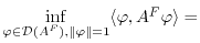
 ,
,(ii) it is the only self-adjoint extension of
whose domain  is contained in
the form domain
is contained in
the form domain  of .
of .
All other self-adjoint extensions have domain not included in
 and a bound
below that is equal or lower, possibly
and a bound
below that is equal or lower, possibly  .
Practise with this phenomena in E23, E24, E25.
.
Practise with this phenomena in E23, E24, E25.(Historical note: In his original paper on self-adjoint extensions von Neumann proved that a semi-bounded operator has semi-bounded extensions whose lower bound is arbitrarily close to the bound of the original operator, and conjectured that extensions exist with the same lower bound. This fact was proved by Friedrichs and Stone.)
T22. Recap on closed semi-bounded quadratic forms, i.e., semi-bounded forms
 (say, with
  )
whose domain
)
whose domain  is complete under the scalar product
  .
.(i) Closure of a form, examples of non-closed / non-closable forms. The form
associated
to a symmetric operator
bounded below (see T21) is closed and bounded below.(ii) A closed semi-bounded quadratic form
identifies a unique self-adjoint operator
such that 
 .
has domain
.
has domain  and acts as
  . The
fact that
. The
fact that  is dense in
  and
and  is uniquely determined follows from Riesz' lemma (and from the
closedness
and symmetry of ).
The fact that is
symmetric follows from the symmetry of .
The fact that
is uniquely determined follows from Riesz' lemma (and from the
closedness
and symmetry of ).
The fact that is
symmetric follows from the symmetry of .
The fact that  follows from the self-adjointness of the bounded linear operator
  ,
which is easier to check and follows again from Riesz' lemma.
,
which is easier to check and follows again from Riesz' lemma.(iii) Thus: there always exist closed extensions of a symmetric operator
(for instance,  )
although it is possible that none of these is self-adjoint, while
semi-bounded forms need not have any closed extensions, but when they
have and are semi-bounded, they are the quadratic forms associated with
self-adjoint operators.
)
although it is possible that none of these is self-adjoint, while
semi-bounded forms need not have any closed extensions, but when they
have and are semi-bounded, they are the quadratic forms associated with
self-adjoint operators.(iv) A closed semi-bounded quadratic form
is
bounded iff the associated self-adjoint operator
is, in which case  (it follows by polarisation). This also proves that
  for any
symmetric operator ,
thus extending the same formula discussed in T6 to the unbounded case.
(Note that this formula is wrong if is
not symmetric!)
for any
symmetric operator ,
thus extending the same formula discussed in T6 to the unbounded case.
(Note that this formula is wrong if is
not symmetric!)T21. Recap on quadratic forms on a Hilbert space
.
(i) Form domain, symmetric forms, forms bounded below (they are
automatically symmetric if
is complex). (ii) The form associated with a symmetric operator
bounded below (say,  ,
where
,
where  ): it's the
quadratic form
with domain given by the
completion of (the domain of )
with respect to the scalar product
): it's the
quadratic form
with domain given by the
completion of (the domain of )
with respect to the scalar product  and defined by
 .
One has
.
One has  and
and 
 . , often denoted also
by
. , often denoted also
by  , is called the form domain of .
Important: the form is
closed (see T22) and bounded below.
Practise with E22, E23.
, is called the form domain of .
Important: the form is
closed (see T22) and bounded below.
Practise with E22, E23.T20. A useful criterion for a symmetric operator
to
have self-adjoint extensions (von Neumann): if there exists a
conjugation  such that
  and
and  ,
then
has equal deficiency indices and therefore has self-adjoint extensions.
Recall that a conjugation
,
then
has equal deficiency indices and therefore has self-adjoint extensions.
Recall that a conjugation  is an antilinear
map that preserves norm and such that
is an antilinear
map that preserves norm and such that  . To apply this criterion to Schrödinger
operators
. To apply this criterion to Schrödinger
operators  (
( real-valued potential) just choose the complex conjugation.
T19. A message from class: different self-adjoint extensions correspond to different physics. See it in the easy example of the motion by translations on
![$ [0,1]$](latex2html/SS11-MQM2-latex2html/SS11-MQM2-latex2html/img224.png) :
the generator is a self-adjoint extension of
:
the generator is a self-adjoint extension of  (see E17, E18), unitarity still leaves the freedom of choosing the
phase of the wave packet as it comes in at zero, by the superposition
principle all functions must change by the same phase when they come
back in. Thus, the different translations are just given by specifying
(see E17, E18), unitarity still leaves the freedom of choosing the
phase of the wave packet as it comes in at zero, by the superposition
principle all functions must change by the same phase when they come
back in. Thus, the different translations are just given by specifying  ,
,
 ,
and by requiring that all reasonable wave packets
,
and by requiring that all reasonable wave packets  satisfy
 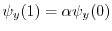 for all ``times''
  .
.T18. Recap on symmetric/self-adjoint extensions of a closed symmetric operator
. (i) The closed symmetric extensions
 of
are
restrictions of
of
are
restrictions of  :
:
 . Thus, one needs to control the
structure of the domain of .
One has
. Thus, one needs to control the
structure of the domain of .
One has  where
where  are
the deficiency spaces of and
the direct sum is with respect to the scalar product
are
the deficiency spaces of and
the direct sum is with respect to the scalar product 
 (in
partic., ,
(in
partic., ,  ,
and
,
and  are all closed w.r.t. this scalar product).
(ii) The closed symmetric extensions are in one-to-one correspondence with partial isometries
 . (A
partial isometry is a bounded linear map
. (A
partial isometry is a bounded linear map  such that
 ![$ (\mathrm{Ker}U)^\perp\xrightarrow[]{U}\mathrm{Ran}U$](latex2html/SS11-MQM2-latex2html/SS11-MQM2-latex2html/img208.png) is
norm-preserving; this implies that
is
norm-preserving; this implies that  too is a partial isometry, since
 ![$ \mathrm{Ran}U\xrightarrow[]{U^*}(\mathrm{Ker}U)^\perp$](latex2html/SS11-MQM2-latex2html/SS11-MQM2-latex2html/img210.png) is norm-preserving; in partic., if
is norm-preserving; in partic., if  then
then  is
an isometry in the usual sense.)
is
an isometry in the usual sense.)(iii) If
is
such an isometry, with  , then the corresponding
closed symmetric extension
, then the corresponding
closed symmetric extension  has domain
  and
action
and
action 
 .
.(iv) If
 then the deficiency indices of
are
then the deficiency indices of
are  . (Recall:
 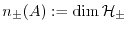 ,
the deficiency indices of .)
,
the deficiency indices of .)(v) Thus,
iff  .
.(vi)
has self-adjoint extensions iff  .
In this case each extension is labelled by a
unitary map .
.
In this case each extension is labelled by a
unitary map .(vii) If either
 or
or  , then
has no non-trivial symmetric extensions ( is
"maximally symmetric").
Practise with E18, E19, E20, E21.
, then
has no non-trivial symmetric extensions ( is
"maximally symmetric").
Practise with E18, E19, E20, E21.T17. Review from class: the step-by-step determination of
 and
and  ,
where
,
where  ,
,
![$ \mathcal{D}(A_0)=\{f\vert f\in C^1([0,1])\,,f(0)=f(1)=0\}$](latex2html/SS11-MQM2-latex2html/SS11-MQM2-latex2html/img183.png) .
General comment: symmetry is easy to check (in case of differential
operators it usually boils down to integration by parts), computing the
adjoint is a non-trivial job even in simple situations. However,
self-adjointness is a much stronger property than symmetry, which
justifies the additional effort needed to prove it.
.
General comment: symmetry is easy to check (in case of differential
operators it usually boils down to integration by parts), computing the
adjoint is a non-trivial job even in simple situations. However,
self-adjointness is a much stronger property than symmetry, which
justifies the additional effort needed to prove it.T16. Recap: symmetry (hermiticity) vs self-adjointness.
(i)
 symmetric means
(ii)
closed and symmetric means 
(iii)
self-adjoint means 
(iv)
essentially self-adjoint means  (and its unique self-adjoint extension is
  ).
). (v) The basic criterion for the self-adjointess of a symmetric operator
on
a Hilbert space :
is
self-adjoint iff
is closed and  ,
equivalently, iff
,
equivalently, iff 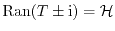 .
. (vi) Criterion for the essential self-adjointess of a symmetric operator
on
a Hilbert space :
is
essentially self-adjoint iff ,
equivalently, iff  are dense in .
T15. New phenomena involving unbounded operators on a Hilbert space with respect to the bounded case:
(i) If
is unbounded,
 may
not be densely defined (example:
may
not be densely defined (example:  ,
,
 ;
then
;
then  and
and  ).
).(ii) If unbounded,
may not be closed (the closure of ,
if it exists, is the unique operator  satisfying
  and is the simplest and
smallest extension of ).
and is the simplest and
smallest extension of ). (iii) If densely defined,
is
closable iff
is densely defined, in which case  .
.T14. Unboundedness is "unavoidable". Position and momentum are unbounded observables. The energy of the harmonic oscillator is an unbounded observable. The Hellinger-Toepliz theorem (follows from Closed Graph).
T13. Recap: the functional calculus for bounded Borel functions of bounded self-adjoint operators on a Hilbert space. The key point is to establish the identity
 for polynomials
  (the rest is just Weiestrass + B.L.T. + bla bla), and it is here that
the self-adjointness of is
crucially needed.
(the rest is just Weiestrass + B.L.T. + bla bla), and it is here that
the self-adjointness of is
crucially needed.T12. The Weyl's criterion. Let
be a bounded, self-adjoint operator on a Hilbert space.  iff there
exists a sequence
iff there
exists a sequence  of
normalised vectors
of
normalised vectors  such that
  as
as  .
See also exercise
3 in FA2, SoSe2009.
.
See also exercise
3 in FA2, SoSe2009.T11. Message from class: the spectral theory of compact operators on a Hilbert space has many similarities with the spectral theory on finite-dimensional spaces (for example, with the possible exception of zero, each eigenvalue of a compact operator has finite multiplicity). However, there are compact operators with no eigenvalues. For example, the Volterra operator [E5]. Or the operator
 ,
,
 :
is compact and
:
is compact and  since
since  is not bounded, however
has no eigenvalues. On the other hand, every non-zero compact and
self-adjoint operator on
a Hilbert space has a non-zero eigenvalue, since either
is not bounded, however
has no eigenvalues. On the other hand, every non-zero compact and
self-adjoint operator on
a Hilbert space has a non-zero eigenvalue, since either  or
or  is an eigenvalue.
T10. Review of useful identities and estimates involving resolvents:
(i)

(ii)


(iii)

(iv)
 for
for 
(v)
 for
for  (the Neumann series)
(vi)

(vii) if
is self-adjoint then 
T9. Misc on orthogonal projections on a Hilbert space. Definition:
 .
.
 is
closed. acts as
the identity on its image and as the zero operator on the orthogonal to
its image. The Projection Theorem establishes a 1:1
correspondence between orthogonal projections and closed subspaces.
Also:
is
closed. acts as
the identity on its image and as the zero operator on the orthogonal to
its image. The Projection Theorem establishes a 1:1
correspondence between orthogonal projections and closed subspaces.
Also:  ,
is normal,
,
is normal,  .
Spectrum:
.
Spectrum:  .
Resolvent:
.
Resolvent:  .
To practise further with orthogonal projections:
.
To practise further with orthogonal projections:(i) Exercise 24, exercise 44, problem 18 in FA, SoSe2010.
(ii) Given two orthogonal projections  ,
,
 ,
one has
,
one has  iff
iff  , in which case they commute
and
, in which case they commute
and  is also an orthogonal projection.
(iii) Given two orthogonal projections ,, exists and is equal to the orthogonal projection onto
  . (Hint:
use the monotonicity of
. (Hint:
use the monotonicity of  .)
.)
T8. Hilbert adjoint vs Banach adjoint. Comparison between the two definitions given in class. Examples (make sure you can work them out again!):
(i) the adjoint of the
 right shift (see [E2.(v)]) is the
  left shift
(ii) the adjoint of the
 Fourier transform (i.e., on test
functions), is the
Fourier transform (i.e., on test
functions), is the  Fourier transform (i.e., on
distributions)
Fourier transform (i.e., on
distributions)(iii) in [E5] we determined the adjoint of the Volterra integral operator
(iv) a multiplication operator with a bounded measurable funct. is selfadjoint in

(v) the adjoint of the Hilbert-Schmidt integral operator [E1.(iv)] acts as

T7. Misc on bounded linear operators on a Hilbert space. One has
 , whence
(Projection Theorem)
, whence
(Projection Theorem) .
If
is normal,
.
If
is normal, 


 . Recall the unique decomposition
  with
with
 and
and  . In
partic., is
normal iff
and
commute, is
unitary iff it is normal and
. In
partic., is
normal iff
and
commute, is
unitary iff it is normal and  .
.T6. Recall that a bounded linear operator
on a Hilbert space is known when one knows all its matrix elements  , and
, and 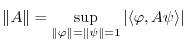 . Via
polarisation
can be reconstructed by its expectations
. Via
polarisation
can be reconstructed by its expectations  . In partic.,
is
equivalent to
. In partic.,
is
equivalent to 
 , and via polarisation+parallelogram law
it follows that the norm of a self-adjoint operator is given by (very
useful!).
, and via polarisation+parallelogram law
it follows that the norm of a self-adjoint operator is given by (very
useful!).
T5. The subadditivity argument needed in the proof (given in class) of the spectral radius formula. Note that the proof given for self-adjoint operators extends to normal operators.
T4. Picture, in the complex plane, of the resolvent set and of the spectrum of a bounded linear operator. The generic case (make sure you can draw it!). For self-adjoint operators the spectrum is on the real line, for unitary operators it is on the unit circle.
T3. A chain of Banach-space theorems (mentioned in class, used ubiquitously): Uniform Boundedness (aka Banach-Steinhaus), Open Mapping, Inverse Mapping, Closed Graph. The underlying Banach structure is crucial: see, e.g., the provocation in problem 42 in FA, SoSe2010. To play a bit with these theorems, look up exercise 44, problem 37, problem 42, and problem 4 (final test) in FA, SoSe2010.
T2. The Riesz Lemma (recap). The proof is based on the Projection Theorem. Corollary: a bounded sesquilinear form identifies uniquely a bounded linear operator:
. Note
that the
orthogonal complement
to the kernel of a bounded linear functional is at most
one-dimensional. T1. The Projection Theorem
 .
We
gave the proof in
Functional Analysis (see e.g. exercise
3 in FA, SoSe2010). Recall that in infinite dimensions the proof
exploits the fact that
.
We
gave the proof in
Functional Analysis (see e.g. exercise
3 in FA, SoSe2010). Recall that in infinite dimensions the proof
exploits the fact that  is closed (of course!) and the
parallelogram law
(this is a Hilbert-space-only feature! see, e.g., exercise
20 in FA, SoSe2010).
is closed (of course!) and the
parallelogram law
(this is a Hilbert-space-only feature! see, e.g., exercise
20 in FA, SoSe2010).