|
|
Date: January 17, 2007.
Acknowledgements. The Minlog system has been under development since around 1990. My sincere thanks go to the many contributors: Holger Benl (Dijkstra algorithm, inductive data types), Ulrich Berger (very many contributions), Michael Bopp (program development by proof transformation), Wilfried Buchholz (translation of classical proof into intuitionistic ones), Laura Crosilla (tutorial), Matthias Eberl (normalization by evaluation), Dan Hernest (functional interpretation), Felix Joachimski (many contributions, in particular translation of classical proofs into intuitionistic ones, producing Tex output, documentation), Ralph Matthes (documentation), Karl-Heinz Niggl (program development by proof transformation), Jaco van de Pol (experiments concerning monotone functionals), Martin Ruckert (many contributions, in particular the MPC tool), Robert Stärk (alpha equivalence), Monika Seisenberger (many contributions, including inductive definitions and translation of classical proofs into intuitionistic ones), Klaus Weich (proof search, the Fibonacci numbers example), Wolfgang Zuber (documentation).
Intro
We now describe in more details some of these features.
1.1. Simultaneous free algebras. A free algebra is given by constructors, for instance zero and successor for the natural numbers. We want to treat other data types as well, like lists and binary trees. When dealing with inductively defined sets, it will also be useful to explicitely refer to the generation tree. Such trees are quite often countably branching, and hence we allow infinitary free algebras from the outset.
The freeness of the constructors is expressed by requiring that their ranges are disjoint and that they are injective. Moreover, we view the free algebra as a domain and require that its bottom element is not in the range of the constructors. Hence the constructors are total and non-strict. For the notion of totality cf. [12, Chapter 8.3].
In our intended semantics we do not require that every semantic object is the denotation of a closed term, not even for finitary algebras. One reason is that for normalization by evaluation (cf. [4]) we want to allow term families in our semantics.
To make a free algebra into a domain and still have the constructors injective and with disjoint ranges, we model e.g. the natural numbers as shown in Figure 1.
Notice that for more complex algebras we usually need many more “infinite” elements; this is a consequence of the closure of domains under suprema. To make dealing with such complex structures less annoying, we will normally restrict attention to the total elements of a domain, in this case – as expected – the elements labelled 0, S0, S(S0) etc.
1.2. Partial continuous functionals. As already mentioned, the (mathematically correct) domains of computable functionals have been identified by Scott and Ershov as the partial continuous functionals; cf. [12]. Since we want to deal with computable functionals in our theory, we consider it as mandatory to accommodate their domains. This is also true if one is interested in total functionals only; they have to be treated as particular partial continuous functionals. We will make use of predicate constants Totalρ with the total functionals of type ρ as the intended meaning. To make formal arguments with quantifiers relativized to total objects more managable, we use a special sort of variables intended to range over such objects only. For example, n0,n1,n2,…,m0,… range over total natural numbers, and nˆ0,nˆ1,nˆ2,… are general variables. This amounts to an abbreviation of
∀ .Totalρ( .Totalρ( ) → A ) → A | by | ∀xA, | |||||
∃ .Totalρ( .Totalρ( ) ∧ A ) ∧ A | by | ∃xA. |
1.3. Primitive recursion, computable functionals. The elimination constants corresponding to the constructors are called primitive recursion operators ℛ. They are described in detail in Section 4. In this setup, every closed term reduces to a numeral.
However, we shall also use constants for rather arbitrary computable functionals, and axiomatize them according to their intended meaning by means of rewrite rules. An example is the general fixed point operator fix, which is axiomatized by fixF = F(fixF). Clearly then it cannot be true any more that every closed term reduces to a numeral. We may have non-terminating terms, but this just means that not always it is a good idea to try to normalize a term.
An important consequence of admitting non-terminating terms is that our notion of proof is not decidable: when checking e.g. whether two terms are equal we may run into a non-terminating computation. But we still have semi-decidability of proofs, i.e., an algorithm to check the correctness of a proof that can only give correct results, but may not terminate. In practice this is sufficient.
To avoid this somewhat unpleasant undecidability phenomenon, we may also view our proofs as abbreviated forms of full proofs, with certain equality arguments left implicit. If some information sufficient to recover the full proof (e.g. for each node a bound on the number of rewrite steps needed to verify it) is stored as part of the proof, then we retain decidability of proofs.
1.4. Decidable predicates, axioms for predicates. As already mentioned, decidable predicates are viewed via boolean valued functions, hence the rewrite mechanism applies to them as well.
Equality is decidable for finitary algebras only; infinitary algebras are to be treated similarly to arrow types. For infinitary algebras (extensional) equality is a predicate constant, with appropriate axioms. In a finitary algebra equality is a (recursively defined) program constant. Similarly, existence (or totality) is a decidable predicate for finitary algebras, and given by predicate constants Totalρ for infinitary algebras as well as composed types. The axioms are listed in Subsection 8.2 of Section 8.
1.5. Minimal logic, proof transformation. For generalities about minimal logic cf. [13]. A concise description of the theory behind the present implementation can be found in “Minimal Logic for Computable Functions” which is available on the Minlog page www.minlog-system.de.
1.6. Comparison with Coq and Isabelle.
SS:Coq
The Isabelle/HOL system of Paulson and Nipkow has its roots in Church’s theory of simple types and Hilbert’s Epsilon calculus. It is an inherently classical system; however, since many proofs in fact use constructive arguments, in is conceivable that program extraction can be done there as well. This has been explored by Berghofer in his thesis [6].
Compared with the Minlog system, the following points are of interest.
S:Types
We have type constants atomic, existential, prop and nulltype. They will be used to assign types to formulas. E.g. ∀nn = 0 receives the type nat → atomic, and ∀n,m∃k n + m = k receives the type nat → nat → existential. The type prop is used for predicate variables, e.g. R of arity nat,nat -> prop. Types of formulas will be necessary for normalization by evaluation of proof terms. The type nulltype will be useful when assigning to a formula the type of a program to be extracted from a proof of this formula. Types not involving the types atomic, existential, prop and nulltype are called object types.
Type variable names are alpha,beta…; alpha is provided by default. To have infinitely many type variables available, we allow appended indices: alpha1,alpha2,alpha3… will be type variables. The only type constants are atomic,existential,prop and nulltype.
2.1. Generalitites for substitutions, type substitutions.
SS:GenSubst
| (make-substitution args vals) | |||||
| (make-substitution-wrt arg-val-equal? args vals) | |||||
| (make-subst arg val) | |||||
| (make-subst-wrt arg-val-equal? arg val) | |||||
| empty-subst |
Composition ϑσ of two substitutions
| ϑ | = ((x1 s1)…(xm sm)), | ||
| σ | = ((y1 t1)…(yn tn)) |
| (compose-substitutions-wrt | substitution-proc arg-equal? | ||||
| arg-val-equal? subst1 subst2) |
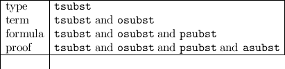
We shall have occasion to use these general substitution procedures for the following kinds of substitutions
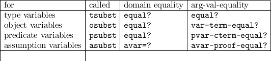
The following substitutions will make sense for a
In particular, for type substitutions tsubst we have
| (type-substitute type tsubst) | |||||
| (type-subst type tvar type1) | |||||
| (compose-t-substitutions tsubst1 tsubst2) |
| (display-t-substitution tsubst) |
2.2. Simultaneous free algebras as base types.
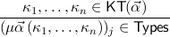
We allow the formation of inductively generated types μ
 , where
 = α1,…,αn is a list of distinct type variables, and
  is a list of “constructor
types” whose argument types contain α1,…,αn in strictly positive positions
only.
is a list of “constructor
types” whose argument types contain α1,…,αn in strictly positive positions
only.
For instance, μα(α,α → α) is the type of natural numbers; here the list (α,α → α) stands for two generation principles: α for “there is a natural number” (the number 0), and α → α for “for every natural number there is another one” (its successor).
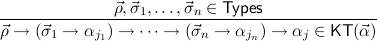
Let an infinite supply of type variables α,β be given. Let  = (αj)j=1,…,m be a
list of distinct type variables. Types ρ,σ,τ,μ,ν ∈ Types and constructor types
κ ∈ KT(
= (αj)j=1,…,m be a
list of distinct type variables. Types ρ,σ,τ,μ,ν ∈ Types and constructor types
κ ∈ KT( ) are defined inductively as follows.
 (n ≥ 0) (n ≥ 0) | |||
 (n ≥ 1, j = 1,…,m) (n ≥ 1, j = 1,…,m) 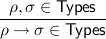 |
 is short for a list ρ1,…,ρk (k ≥ 0) of types and
  → σ means
ρ1 →
→ σ means
ρ1 → → ρk → σ, associated to the right. We shall use μ,ν for types
of the form (μ
→ ρk → σ, associated to the right. We shall use μ,ν for types
of the form (μ (κ1,…,κn))j only, and for types
  = (τj)j=1,…,m and a
constructor type κ =
= (τj)j=1,…,m and a
constructor type κ =  → (
→ ( 1 → αj1) →
 → (
→ ( n → αjn) → αj ∈ KT(
 )
let
)
let
![κ[⃗τ ] := ⃗ρ → (⃗σ1 → τj1) → ⋅⋅⋅ → (⃗σn → τjn) → τj.](ref26x.png)
Examples.
| unit | := μαα, | ||||||
| boole | := μα (α,α), | ||||||
| nat | := μα (α,α → α), | ||||||
| ytensor(α1)(α2) | := μα.α1 → α2 → α, | ||||||
| ypair(α1)(α2) | := μα.(unit → α1) → (unit → α2) → unit → α, | ||||||
| yplus(α1)(α2) | := μα.(α1 → α,α2 → α), | ||||||
| list(α1) | := μα (α,α1 → α → α), | ||||||
| (tree,tlist) | := μ(α,β)(α,β → α,β,α → β → β), | ||||||
| btree | := μα (α,α → α → α), | ||||||
| 𝒪 | := μα (α,α → α,(nat → α) → α), | ||||||
| 𝒯0 | := nat, | ||||||
| 𝒯n+1 | := μα (α,(𝒯n → α) → α). |
To add and remove names for type variables, we use
| (add-tvar-name name1 ...) | |||
| (remove-tvar-name name1 ...) |
| (make-tvar index name) | constructor | ||||||
| (tvar-to-index tvar) | accessor | ||||||
| (tvar-to-name tvar) | accessor | ||||||
| (tvar? x). |
| (new-tvar type) |
To introduce simultaneous free algebras we use

An example is
(add-param-algs
(list "labtree" "labtlist") ’alg-typeop 2 ’("LabLeaf" "alpha1=>labtree") ’("LabBranch" "labtlist=>alpha2=>labtree") ’("LabEmpty" "labtlist") ’("LabTcons" "labtree=>labtlist=>labtlist" pairscheme-op)) |
This simultaneously introduces the two free algebras labtree and labtlist, both finitary, whose constructors are LabLeaf, LabBranch, LabEmpty and LabTcons (written as an infix pair operator, hence right associative). The constructors are introduced as “self-evaluating” constants; they play a special role in our semantics for normalization by evaluation.
In case there are no parameters we use add-algs, and in case there is no need for a simultaneous definition we use add-alg or add-param-alg.
For already introduced algebras we need constructors and accessors
| (alg-form? x) | incomplete test | ||||||
| (alg? x) | complete test | ||||||
| (finalg? type) | incomplete test | ||||||
| (ground-type? x) | incomplete test |
We require that there is at least one nullary constructor in every free algebra; hence, it has a “canonical inhabitant”. For arbitrary types this need not be the case, but occasionally (e.g. for general logical problems, like to prove the drinker formula) it is useful. Therefore
| (make-inhabited type term1 ...) |

which returns the canonical inhabitant; it is an error to apply this procedure to a non-inhabited type. We do allow non-inhabited types to be able to implement some aspects of [7, 1]
To remove names for algebras we use
| (remove-alg-name name1 ...) |
Examples. Standard examples for finitary free algebras are the type nat of unary natural numbers, and the type btree of binary trees. The domain ℐnat of unary natural numbers is defined (as in [4]) as a solution to a domain equation.
We always provide the finitary free algebra unit consisting of exactly one element, and boole of booleans; objects of the latter type are (cf. loc. cit.) true, false and families of terms of this type, and in addition the bottom object of type boole.
Tests:
| (arrow-form? type) | |||
| (star-form? type) | |||
| (object-type? type) |
We also need constructors and accessors for arrow types
| (make-arrow arg-type val-type) | constructor | ||||||
| (arrow-form-to-arg-type arrow-type) | accessor | ||||||
| (arrow-form-to-val-type arrow-type) | accessor |
| (make-star type1 type2) | constructor | ||||||
| (star-form-to-left-type star-type) | accessor | ||||||
| (star-form-to-right-type star-type) | accessor. |
| (mk-arrow type1 ... type) | |||||||
| (arrow-form-to-arg-types type <n>) | all (first n) argument types | ||||||
| (arrow-form-to-final-val-type type) | type of final value. |
| (type? x) | |||
| (type-to-string type). |
Implementation. Type variables are implemented as lists:

Variables
In most cases we need to argue about existing (i.e. total) objects only. For the notion of totality we have to refer to [12, Chapter 8.3]; particularly relevant here is exercise 8.5.7. To make formal arguments with quantifiers relativized to total objects more managable, we use a special sort of variables intended to range over such objects only. For example, n0,n1,n2,…,m0,… range over total natural numbers, and nˆ0,nˆ1,nˆ2,… are general variables. We say that the degree of totality for the former is 1, and for the latter 0.
n,m for variables of type nat), we use
| (add-var-name name1 ... type) | |||
| (remove-var-name name1 ... type) | |||
| (default-var-name type). |
We need a constructor, accessors and tests for variables.
equal? is a valid test for equality of variables. Moreover, it is guaranteed that parsing a displayed variable reproduces the variable; the converse need not be the case (we may want to convert it into some canonical form).For convenience we have the function
| (mk-var type <index> <t-deg> <name>). |
| (default-var-name type) |
Using the empty string as the name, we can create so called numerated variables. We further require that we can test whether a given variable belongs to those special ones, and that from every numerated variable we can compute its index:
| (numerated-var? var) | |||
| (numerated-var-to-index numerated-var). |

with inverses var-to-type, numerated-var-to-index and var-to-t-deg.
Although these functions look like an ad hoc extension of the interface that is convenient for normalization by evaluation, there is also a deeper background: these functions can be seen as the “computational content” of the well-known phrase “we assume that there are infinitely many variables of every type”. Giving a constructive proof for this statement would require to give infinitely many examples of variables for every type. This of course can only be done by specifying a function (for every type) that enumerates these examples. To make the specification finite we require the examples to be given in a uniform way, i.e. by a function of two arguments. To make sure that all these examples are in fact different, we would have to require make-var to be injective. Instead, we require (classically equivalent) make-var to be a bijection on its image, as again, this can be turned into a computational statement by requiring that a witness (i.e. an inverse function) is given.
Finally, as often the exact knowledge of infinitely many variables of every type is not needed we require that, either by using the above functions or by some other form of definition, functions
| (type-to-new-var type) | |||
| (type-to-new-partial-var type) |
Occasionally we may want to create a new variable with the same name (and degree of totality) as a given one. This is useful e.g. for bound renaming. Therefore we supply
| (var-to-new-var var). |
Implementation. Variables are implemented as lists:

Pconst
The latter are built into the system: recursion operators for arbitrary algebras,
equality and existence operators for finitary algebras, and existence elimination.
They are typed in parametrized form, with the actual type (or formula) given
by a type (or type and formula) substitution that is also part of the
constant. For instance, equality is typed by α → α → boole and a type
substitution α ρ. This is done for clarity (and brevity, e.g. for large ρ in the
example above), since one should think of the type of a constant in this
way.
ρ. This is done for clarity (and brevity, e.g. for large ρ in the
example above), since one should think of the type of a constant in this
way.
For constructors and for constants with fixed rules, by efficiency reasons we want to keep the object denoted by the constant (as needed for normalization by evaluation) as part of it. It depends on the type of the constant, hence must be updated in a given proof whenever the type changes by a type substitution.
4.1. Rewrite and computation rules for program constants.
SS:RewCompRules

 N are given, where FV(N) ⊆ FV(
 ) and c
 , N have the
same type (not necessarily a ground type). Moreover, for any two rules c
, N have the
same type (not necessarily a ground type). Moreover, for any two rules c
 N
and c
N
and c ′
′ N′ we require that
  and
and  ′ are of the same length, called the arity
of c. The rules are divided into computation rules and proper rewrite rules. They
must satisfy the requirements listed in [4]. The idea is that a computation
rule can be understood as a description of a computation in a suitable
semantical model, provided the syntactic constructors correspond to
semantic ones in the model, whereas the other rules describe syntactic
transformations.
′ are of the same length, called the arity
of c. The rules are divided into computation rules and proper rewrite rules. They
must satisfy the requirements listed in [4]. The idea is that a computation
rule can be understood as a description of a computation in a suitable
semantical model, provided the syntactic constructors correspond to
semantic ones in the model, whereas the other rules describe syntactic
transformations.
There a more general approach was used: one may enter into components of
products. Then instead of one arity one needs several “type informations”  → σ
with
→ σ
with  a list of types, 0’s and 1’s indicating the left or right part of a product
type. For example, if c is of type τ → (τ → τ → τ) × (τ → τ), then the rules
cy0xx
a list of types, 0’s and 1’s indicating the left or right part of a product
type. For example, if c is of type τ → (τ → τ → τ) × (τ → τ), then the rules
cy0xx a and cy1
 b are admitted, and c comes with the type informations
(τ,0,τ,τ → τ) → τ and (τ,1) → (τ → τ). – However, for simplicity we only deal
with a single arity here.
b are admitted, and c comes with the type informations
(τ,0,τ,τ → τ) → τ and (τ,1) → (τ → τ). – However, for simplicity we only deal
with a single arity here.
Given a set of rewrite rules, we want to treat some rules - which we call computation rules - in a different, more efficient way. The idea is that a computation rule can be understood as a description of a computation in a suitable semantical model, provided the syntactic constructors correspond to semantic ones in the model, whereas the other rules describe syntactic transformations.
In order to define what we mean by computation rules, we need the notion of a constructor pattern. These are special terms defined inductively as follows.
 is of ground type, then c
 is a constructor pattern.
From the given set of rewrite rules we choose a subset Comp with the following properties.

 Q ∈ Comp, then P1,…,Pn are constructor patterns or
projection markers.
Q ∈ Comp, then P1,…,Pn are constructor patterns or
projection markers.

 Q ∈ Comp, then every variable
in c
Q ∈ Comp, then every variable
in c occurs only once in c
 .
.

 M and
c
M and
c
 N in Comp the left hand sides c
 and c
and c are non-unifiable.
We write c
 compQ to indicate that the rule is in Comp. All other rules will be
called (proper) rewrite rules, written c
compQ to indicate that the rule is in Comp. All other rules will be
called (proper) rewrite rules, written c
 rewK.
rewK.
In our reduction strategy computation rules will always be applied first, and
since they are non-overlapping, this part of the reduction is unique. However,
since we allowed almost arbitrary rewrite rules, it may happen that in case no
computation rule applies a term may be rewritten by different rules  Comp. In
order to obtain a deterministic procedure we then select the first applicable
rewrite rule (This is a slight simplification of [4], where special functions selc were
used for this purpose).
Comp. In
order to obtain a deterministic procedure we then select the first applicable
rewrite rule (This is a slight simplification of [4], where special functions selc were
used for this purpose).
4.2. Recursion over simultaneous free algebras.
SS:RecSFA
 = μ
= μ
 corresponds to two
sorts of constants. With the constructors constri
corresponds to two
sorts of constants. With the constructors constri : κi[
: κi[ ] we can construct
elements of a type μj, and with the recursion operators ℛμj
] we can construct
elements of a type μj, and with the recursion operators ℛμj ,
, we can
construct mappings from μj to τj by recursion on the structure of
we can
construct mappings from μj to τj by recursion on the structure of  . So in
(Rec arrow-types), arrow-types is a list μ1 → τ1,…,μk → τk. Here
μ1,…,μk are the algebras defined simultaneously and τ1,…,τk are the result
types.
. So in
(Rec arrow-types), arrow-types is a list μ1 → τ1,…,μk → τk. Here
μ1,…,μk are the algebras defined simultaneously and τ1,…,τk are the result
types.
For convenience in our later treatment of proofs (when we want to normalize a proof by (1) translating it into a term, (2) normalizing this term and (3) translating the normal term back into a proof), we also allow all-formulas ∀x1μ1A1,…,∀xkμkAk instead of arrow-types: they are treated as μ1 → τ(A1), ..., μk → τ(Ak) with τ(Aj) the type of Aj.
Recall the definition of types and constructor types in Section 2, and the
examples given there. In order to define the type of the recursion operators
w.r.t.  = μ
= μ
 and result types
  , we first define for

the step type
δi , , := :=  → → | ( 1 → μj1) →
 → ( → ( n → μjn) → n → μjn) → | ||
( 1 → τj1) → 1 → τj1) → → ( → ( n → τjn) → τj. n → τjn) → τj. |
 ,(
,( 1 → μj1),…,(
 n → μjn) correspond to the components of the object of
type μj under consideration, and (
n → μjn) correspond to the components of the object of
type μj under consideration, and ( 1 → τj1),…,(
 n → τjn) to the previously
defined values. The recursion operator ℛμj
n → τjn) to the previously
defined values. The recursion operator ℛμj ,
, has type

We will often write ℛj ,
, for ℛμj
 ,
, , and omit the upper indices
  ,
, when
they are clear from the context. In case of a non-simultaneous free algebra, i.e. of
type μα (κ), for ℛμμ,τ we normally write ℛμτ.
when
they are clear from the context. In case of a non-simultaneous free algebra, i.e. of
type μα (κ), for ℛμμ,τ we normally write ℛμτ.
A simple example for simultaneous free algebras is

The constructors are
| Leaftree := constr 1(tree,tlist), | |||
| Branchtlist→tree := constr 2(tree,tlist), | |||
| Emptytlist := constr 3(tree,tlist), | |||
| Tconstree→tlist→tlist := constr 4(tree,tlist). |
| (const Rec δ1 → δ2 → δ3 → δ4 → tree → α1 | |||||
(α1 τ1,α2 τ1,α2 τ2)) τ2)) | |||||
| with | |||||
| δ1 := α1, | |||||
| δ2 := tlist → α2 → α1, | |||||
| δ3 := α2, | |||||
| δ4 := tree → tlist → α1 → α2 → α2. | |||||
For the external representation (i.e. display) we use the shorter notation

As already mentioned, it is also possible that the object constant Rec comes with formulas instead of types, as the assumption constant Ind below. This is due to our desire not to duplicate code when normalizing proofs, but rather translate the proof into a term first, normalize the term and then translate back into a proof. For the last step we must have the original formulas of the induction operator available.
To see a concrete example, let us recursively define addition +: tree → tree → tree and ⊕: tlist → tree → tlist. The recursion equations to be satisfied are
| + Leaf | = λaa, | ||||||
| + (Branchbs) | = λa.Branch(⊕bs a), | ||||||
| ⊕ Empty | = λaEmpty, | ||||||
| ⊕ (Tconsbbs) | = λa.Tcons(+ba)(⊕bs a). |
| τ1 | := tree → tree, | ||
| τ2 | := tree → tlist. |
| M1 | := λaa, | ||
| M2 | := λbsλgτ2 λa.Branch(g a), | ||
| M3 | := λaEmpty, | ||
| M4 | := λbλbsλfτ1 λgτ2 λa.Tcons(f a)(g a). |
| + | := ℛtree : tree → tree → tree, : tree → tree → tree, | ||
| ⊕ | := ℛtlist : tlist → tree → tlist. : tlist → tree → tlist. |
To explain the conversion relation, it will be useful to employ the following
notation. Let  = μ
= μ
 ,
,

and consider constri
 . Then we write
  P = N1P ,…,NmP for the parameter
arguments N1ρ1,…,Nmρm and
P = N1P ,…,NmP for the parameter
arguments N1ρ1,…,Nmρm and  R = N1R,…,NnR for the recursive arguments
Nm+1
R = N1R,…,NnR for the recursive arguments
Nm+1 1→μj1,…,Nm+n
 n→μjn, and nR for the number n of recursive arguments.
We define a conversion relation  ρ between terms of type ρ by
| (λxM)N |  M[x:=N] M[x:=N] | (1) |
| λx.Mx |  M if x M if x FV(M), M not an abstraction FV(M), M not an abstraction | (2) |
(ℛj , ,  )μj→τj
(constri )μj→τj
(constri  ) ) |  M
i M
i  (ℛj
1 (ℛj
1 , ,  ) ∘ N
1R ) ∘ N
1R … … (ℛ
jn (ℛ
jn , ,  ) ∘ N
nR ) ∘ N
nR | (3) |
 ,
, for ℛμj
 ,
, , and ∘ means composition.
4.3. Internal representation of constants. Every object constant has the internal representation
| (const | object-or-arity name uninst-type-or-formula subst | ||
| t-deg token-type arrow-types-or-repro-formulas), |
(const Compose (α→β)→(β→γ)→α→γ (α ρ,β ρ,β σ,γ σ,γ τ) ...) τ) ...) | |||||
(const Eq α → α → boole (α finalg) ...) finalg) ...) | |||||
(const E α → boole (α finalg…)) finalg…)) | |||||
| (const Ex-Elim ∃xαP(x) → (∀xα.P(x) → Q) → Q | |||||
(α τ,P(α) τ,P(α) {zτ ∣ A},Q {zτ ∣ A},Q { ∣ B }) ...) { ∣ B }) ...) |
Constructor, accessors and tests for all kinds of constants:
tsubst must be restricted to the type variables in uninst-type. arrow-types-or-repro-formulas are only present for the Rec constants. They are needed for the reproduction case.From these we can define
| (const-to-type const) | |||||
| (const-to-tvars const) |
A constructor is a special constant with no rules. We maintain an association list CONSTRUCTORS assigning to every name of a constructor an association list associating with every type substitution (restricted to the type parameters) the corresponding instance of the constructor. We provide
| (constr-name? string) | |||||
| (constr-name-to-constr name <tsubst>) | |||||
| (constr-name-and-tsubst-to-constr name tsubst), |
For given algebras one can display the associated constructors with their types by calling
| (display-constructors alg-name1 ...). |
We also need procedures recovering information from the string denoting a program constant (via PROGRAM-CONSTANTS):
One can display the program constants together with their current computation and rewrite rules by calling
| (display-program-constants name1 ...). |
To add and remove program constants we use
| (add-program-constant name type <rest>) | |||
| (remove-program-constant symbol); |
To add and remove computation and rewrite rules we have
| (add-computation-rule lhs rhs) | |||
| (add-rewrite-rule lhs rhs) | |||
| (remove-computation-rules-for lhs) | |||
| (remove-rewrite-rules-for lhs). |
To generate our constants with fixed rules we use
| (finalg-to-=-const finalg) | equality | ||||||
| (finalg-to-e-const finalg) | existence | ||||||
| (arrow-types-to-rec-const . arrow-types) | recursion | ||||||
| (ex-formula-and-concl-to-ex-elim-const | |||||||
| ex-formula concl) |
Similarly to arrow-types-to-rec-const we also define the procedure all-formulas-to-rec-const. It will be used in to achieve normalization of proofs via translating them in terms.
[Noch einfügen: arrow-types-to-cases-const und zur Behandlung von Beweisen all-formulas-to-cases-const]
S:Psyms
SS:PredVars
Predicate variable names are provided in the form of an association list, which assigns to the names their arities. By default we have the predicate variable bot of arity (arity), called (logical) falsity. It is viewed as a predicate variable rather than a predicate constant, since (when translating a classical proof into a constructive one) we want to substitute for bot.
Often we will argue about Harrop formulas only, i.e. formulas without computational content. For convenience we use a special sort of predicate variables intended to range over comprehension terms with Harrop formulas only. For example, P0,P1,P2,…,Q0,… range over comprehension terms with Harrop formulas, and Pˆ0,Pˆ1,Pˆ2,… are general predicate variables. We say that Harrop degree for the former is 1, and for the latter 0.
We need constructors and accessors for arities
| (make-arity type1 ...) | |||
| (arity-to-types arity) |

We can test whether a string is a name for a predicate variable, and if so compute its associated arity:
| (pvar-name? string) | |||
| (pvar-name-to-arity pvar-name) |
To add and remove names for predicate variables of a given arity (e.g. Q for predicate variables of arity nat), we use
| (add-pvar-name name1 ... arity) | |||
| (remove-pvar-name name1 ...) |
We need a constructor, accessors and tests for predicate variables.
For convenience we have the function
| (mk-pvar arity <index> <h-deg> <name>) |
It is guaranteed that parsing a displayed predicate variable reproduces the predicate variable; the converse need not be the case (we may want to convert it into some canonical form).
SS:PredConsts
Notice that a predicate constant does not change its name under a type substitution; this is in contrast to predicate (and other) variables. Notice also that the parser can infer from the arguments the types ρ1…ρn to be substituted for the type variables in the uninstantiated arity of P.
To add and remove names for predicate constants of a given arity, we use
| (add-predconst-name name1 ... arity) | |||
| (remove-predconst-name name1 ...) |
| (predconst-name? name) | |||||
| (predconst-name-to-arity predconst-name). | |||||
| (predconst-to-string predconst). |
5.3. Inductively defined predicate constants.
SS:IDPredConsts

 . Similarly, we can use predicate variables to
inductively generate predicates μ
. Similarly, we can use predicate variables to
inductively generate predicates μ
 .
.
More precisely, we allow the formation of inductively generated predicates
μ
 , where
  = (Xj)j=1,…,N is a list of distinct predicate variables, and
 = (Ki)i=1,…,k is a list of constructor formulas (or “clauses”) containing
X1,…,XN in strictly positive positions only.
= (Ki)i=1,…,k is a list of constructor formulas (or “clauses”) containing
X1,…,XN in strictly positive positions only.
To introduce inductively defined predicates we use

An example is
(add-ids (list (list "Ev" (make-arity (py "nat")) "algEv")
(list "Od" (make-arity (py "nat")) "algOd")) ’("Ev 0" "InitEv") ’("allnc n.Od n -> Ev(n+1)" "GenEv") ’("Od 1" "InitOd") ’("allnc n.Ev n -> Od(n+1)" "GenOd")) |
This simultaneously introduces the two inductively defined predicate constants Ev and Od, by the clauses given. The presence of an algebra name after the arity (here algEv and algOd) indicates that this inductively defined predicate constant is to have computational content. Then all clauses with this constant in the conclusion must provide a constructor name (here InitEv, GenEv, InitOd, GenOd). If the constant is to have no computational content, then all its clauses must be invariant (under realizability, a.k.a. “negative”).
Here are some further examples of inductively defined predicates:
(add-ids
(list (list "Even" (make-arity (py "nat")) "algEven")) ’("Even 0" "InitEven") ’("allnc n.Even n -> Even(n+2)" "GenEven")) (add-ids (list (list "Acc" (make-arity (py "nat")) "algAcc")) ’("allnc n.(all m.m<n -> Acc m) -> Acc n" "GenAccSup")) (add-ids (list (list "OrID" (make-arity) "algOrID")) ’("Pˆ1 -> OrID" "InlOrID") ’("Pˆ2 -> OrID" "InrOrID")) (add-ids (list (list "EqID" (make-arity (py "alpha") (py "alpha")) "algEqID")) ’("allnc xˆ EqID xˆ xˆ" "GenEqID")) (add-ids (list (list "ExID" (make-arity) "algExID")) ’("allnc xˆ.Qˆ xˆ -> ExID" "GenExID")) (add-ids (list (list "FalsityID" (make-arity) "algFalsityID"))) |
Terms
The if-construct distinguishes cases according to the outer constructor form; the simplest example (for the type boole) is if-then-else. Here we do not want to evaluate all arguments right away, but rather evaluate the test argument first and depending on the result evaluate at most one of the other arguments. This phenomenon is well known in functional languages; e.g. in Scheme the if-construct is called a special form as opposed to an operator. In accordance with this terminology we also call our if-construct a special form. It will be given a special treatment in nbe-term-to-object.
Usually it will be the case that every closed term of an sfa ground type reduces via the computation rules to a constructor term, i.e. a closed term built from constructors only. However, we do not require this.
We have constructors, accessors and tests for variables
| (make-term-in-var-form var) | constructor | ||||||
| (term-in-var-form-to-var term) | accessor, | ||||||
| (term-in-var-form? term) | test, |
| (make-term-in-const-form const) | constructor | ||||||
| (term-in-const-form-to-const term) | accessor | ||||||
| (term-in-const-form? term) | test, |
| (make-term-in-abst-form var term) | constructor | ||||||
| (term-in-abst-form-to-var term) | accessor | ||||||
| (term-in-abst-form-to-kernel term) | accessor | ||||||
| (term-in-abst-form? term) | test, |
| (make-term-in-app-form term1 term2) | constructor | ||||||
| (term-in-app-form-to-op term) | accessor | ||||||
| (term-in-app-form-to-arg term) | accessor | ||||||
| (term-in-app-form? term) | test, |
| (make-term-in-pair-form term1 term2) | constructor | ||||||
| (term-in-pair-form-to-left term) | accessor | ||||||
| (term-in-pair-form-to-right term) | accessor | ||||||
| (term-in-pair-form? term) | test, |
It is convenient to have more general application constructors and accessors available, where application takes arbitrary many arguments and works for ordinary application as well as for component formation.
| (mk-term-in-app-form term term1 ...) | constructor | ||||||
| (term-in-app-form-to-final-op term) | accessor | ||||||
| (term-in-app-form-to-args term) | accessor, |
| (mk-term-in-abst-form var1 ... term). |
Moreover we need
| (term? x) | |||||
| (term=? term1 term2) | |||||
| (terms=? terms1 terms2) | |||||
| (term-to-type term) | |||||
| (term-to-free term) | |||||
| (term-to-bound term) | |||||
| (term-to-t-deg term) | |||||
| (synt-total? term) | |||||
| (term-to-string term). |
6.1. Normalization. We need an operation which transforms a term into its normal form w.r.t. the given computation and rewrite rules. Here we base our treatment on normalization by evaluation introduced in [5], and extended to arbitrary computation and rewrite rules in [4].
For normalization by evaluation we need semantical objects. For an arbitrary ground type every term family of that type is an object. For an sfa ground type, in addition the constructors have semantical counterparts. The freeness of the constructors is expressed by requiring that their ranges are disjoint and that they are injective. Moreover, we view the free algebra as a domain and require that its bottom element is not in the range of the constructors. Hence the constructors are total and non-strict. Then by applying nbe-reflect followed by nbe-reify we can normalize every term, where normalization refers to the computation as well as the rewrite rules.
An object consists of a semantical value and a type.
| (nbe-make-object type value) | constructor | ||||||
| (nbe-object-to-type object) | accessor | ||||||
| (nbe-object-to-value object) | accessor | ||||||
| (nbe-object? x) | test. |
| (nbe-object-apply function-obj arg-obj) |
| (nbe-object-app function-obj arg-obj1 ...) | |||||
| (nbe-object-compose function-obj1 function-obj2) |

where delayed-constr is a procedure of zero arguments which evaluates to this very same constructor. This is necessary to avoid having a cycle (for nullary constructors, and only for those).
| (nbe-pconst-and-tsubst-and-rules-to-object | |||
| pconst tsubst comprules rewrules) |
| (nbe-term-to-object term bindings) | evaluation. |
The interpretation of the program constants requires some auxiliary functions (cf. [4]):
| (nbe-reify object) | reification | ||||||
| (nbe-reflect term) | reflection |
| (nbe-normalize-term term) | normalization, |
The if-form needs a special treatment. In particular, for a full normalization of terms (including permutative conversions), we define a preprocessing step that η expands the alternatives of all if-terms. The result contains if-terms with ground type alternatives only.
6.2. Substitution. Recall the generalities on substitutions in Section 2.1.
We define simultaneous substitution for type and object variables in a term, via tsubst and subst. It is assumed that subst only affects those vars whose type is not changed by tsubst.
In the abstraction case of the recursive definition, the abstracted variable may need to be renamed. However, its type can be affected by tsubst. Then the renaming cannot be made part of subst, because the condition above would be violated. Therefore we carry along a procedure renaming variables, which remembers the renaming of variables done so far.
| (term-substitute term tosubst) | |||||
| (term-subst term arg val) | |||||
| (compose-o-substitutions subst1 subst2) |
Display functions for substitutions are
| (display-substitution subst) | |||
| (substitution-to-string subst) |
S:Formulas
Formulas are built from prime formulas by
Moreover we have classical existential quantification in an arithmetical and a logical form:
| (exca (x1...) formula) | arithmetical version | ||||||
| (excl (x1 ...) formula) | logical version. |
Formulas can be unfolded in the sense that the all classical existential quantifiers are replaced according to their definiton. Inversely a formula can be folded in the sense that classical existential quantifiers are introduced wherever possible.
Comprehension terms have the form (cterm vars formula). Note that formula may contain further free variables.
Tests:
| (quant-prime-form? formula) | |||
| (quant-free? formula). |
We need constructors and accessors for prime formulas
| (make-atomic-formula boolean-term) | |||||
| (make-predicate-formula predicate term1 ...) | |||||
| atom-form-to-kernel | |||||
| predicate-form-to-predicate | |||||
| predicate-form-to-args. |
| (make-imp premise conclusion) | constructor | ||||||
| (imp-form-to-premise imp-formula) | accessor | ||||||
| (imp-form-to-conclusion imp-formula) | accessor, |
| (make-and formula1 formula2) | constructor | ||||||
| (and-form-to-left and-formula) | accessor | ||||||
| (and-form-to-right and-formula) | accessor, |
| (make-tensor formula1 formula2) | constructor | ||||||
| (tensor-form-to-left tensor-formula) | accessor | ||||||
| (tensor-form-to-right tensor-formula) | accessor, |
| (make-all var formula) | constructor | ||||||
| (all-form-to-var all-formula) | accessor | ||||||
| (all-form-to-kernel all-formula) | accessor, |
| (make-ex var formula) | constructor | ||||||
| (ex-form-to-var ex-formula) | accessor | ||||||
| (ex-form-to-kernel ex-formula) | accessor, |
| (make-allnc var formula) | constructor | ||||||
| (allnc-form-to-var allnc-formula) | accessor | ||||||
| (allnc-form-to-kernel allnc-formula) | accessor, |
| (make-exnc var formula) | constructor | ||||||
| (exnc-form-to-var exnc-formula) | accessor | ||||||
| (exnc-form-to-kernel exnc-formula) | accessor, |
| (make-exca var formula) | constructor | ||||||
| (exca-form-to-var exca-formula) | accessor | ||||||
| (exca-form-to-kernel exca-formula) | accessor, |
| (make-excl var formula) | constructor | ||||||
| (excl-form-to-var excl-formula) | accessor | ||||||
| (excl-form-to-kernel excl-formula) | accessor. |
| (imp-form-to-premises-and-final-conclusion formula) | |||||
| (tensor-form-to-parts formula) | |||||
| (all-form-to-vars-and-final-kernel formula) | |||||
| (ex-form-to-vars-and-final-kernel formula) |
| (imp-form-to-premises formula <n>) | all (first n) premises | ||||||
| (imp-form-to-final-conclusion formula <n>) |
It is also useful to have some general procedures working for arbitrary quantified formulas. We provide

To fold and unfold formulas we have
| (fold-formula formula) | |||
| (unfold-formula formula). |
| (classical-formula=? formula1 formula2) | |||
| (formula=? formula1 formula2), |
Morever we need
| (formula-to-free formula), | |||
| (nbe-formula-to-type formula), | |||
| (formula-to-prime-subformulas formula), |
Constructors, accessors and a test for comprehension terms are
| (make-cterm var1 ... formula) | constructor | ||||||
| (cterm-to-vars cterm) | accessor | ||||||
| (cterm-to-formula cterm) | accessor | ||||||
| (cterm? x) | test. |
| (cterm-to-free cterm) | |||
| (cterm=? x) | |||
| (classical-cterm=? x) | |||
| (fold-cterm cterm) | |||
| (unfold-cterm cterm). |
Normalization of formulas is done with
| (normalize-formula formula) | normalization, |
To check equality of formulas we use
| (classical-formula=? formula1 formula2) | |||||
| (formula=? formula1 formula2) |
Display functions for formulas and comprehension terms are
| (formula-to-string formula) | |||||
| (cterm-to-string cterm). |
We can define simultaneous substitution for type, object and predicate variables in a formula, via tsubst, subst and psubst. It is assumed that subst only affects those variables whose type is not changed by tsubst, and that psubst only affects those predicate variables whose arity is not changed by tsubst.
In the quantifier case of the recursive definition, the abstracted variable may need to be renamed. However, its type can be affected by tsubst. Then the renaming cannot be made part of subst, because then the condition above would be violated. Therefore we carry along a procedure rename renaming variables, which remembers the renaming of variables done so far.
We will also need formula substitution to compute the formula of an assumption constant. However, there (type and) predicate variables are (implicitely) considered to be bound. Therefore, we also have to carry along a procedure prename renaming predicate variables, which remembers the renaming of predicate variables done so far.
| (formula-substitute formula topsubst) | |||||
| (formula-subst formula arg val) | |||||
| (cterm-substitute cterm topsubst) | |||||
| (cterm-subst cterm arg val) |
Display functions for predicate substitutions are
| (display-p-substitution psubst) | |||
| (p-substitution-to-string psubst) |
S:AssumptionVarConst
8.1. Assumption variables. Assumption variables are for proofs what variables are for terms. The main difference, however, is that assumption variables have formulas as types, and that formulas may contain free variables. Therefore we must be careful when substituting terms for variables in assumption variables. Our solution (as in Matthes’ thesis [9]) is to consider an assumption variable as a pair of a (typefree) identifier and a formula, and to take equality of assumption variables to mean that both components are equal. Rather than using symbols as identifiers we prefer to use numbers (i.e. indices). However, sometimes it is useful to provide an optional string as name for display purposes.
We need a constructor, accessors and tests for assumption variables.
| (make-avar formula index name) | constructor | ||||||
| (avar-to-formula avar) | accessor | ||||||
| (avar-to-index avar) | accessor | ||||||
| (avar-to-name avar) | accessor | ||||||
| (avar? x) | test | ||||||
| (avar=? avar1 avar2) | test. |
| (mk-avar formula <index> <name>) |
| (formula-to-new-avar formula) |
An assumption constant appears in a proof, as an axiom, a theorem or a global assumption. Its formula is given as an “uninstantiated formula”, where only type and predicate variables can occur freely; these are considered to be bound in the assumption constant. In the proof the bound type variables are implicitely instantiated by types, and the bound predicate variables by comprehension terms (the arity of a comprehension term is the type-instantiated arity of the corresponding predicate variable). Since we do not have type and predicate quantification in formulas, the assumption constant contains these parts left implicit in the proof: tsubst and pinst (which will become a psubst, once the arities of predicate variables are type-instantiated with tsubst).
So we have assumption constants of the following kinds:
To normalize a proof we will first translate it into a term, then normalize the term and finally translate the normal term back into a proof. To make this work, in case of axioms we pass to the term appropriate formulas: all-formulas for induction, an existential formula for existence introduction, and an existential formula together with a conclusion for existence elimination. During normalization of the term these formulas are passed along. When the normal form is reached, we have to translate back into a proof. Then these formulas are used to reconstruct the axiom in question.
Internally, the formula of an assumption constant is split into an uninstantiated formula where only type and predicate variables can occur freely, and a substitution for at most these type and predicate variables. The formula assumed by the constant is the result of carrying out this substitution in the uninstantiated formula. Note that free variables may again occur in the assumed formula. For example, assumption constants axiomatizing the existential quantifier will internally have the form
(aconst Ex-Intro ∀ α. α. ( ( ) →∃ ) →∃ α α ( ( ) (α ) (α τ, τ, (α) (α) { { τ ∣ A})) τ ∣ A})) | |||||
(aconst Ex-Elim ∃ α α ( ( ) → (∀ ) → (∀ α. α. ( ( ) → ) → ) → ) → | |||||
(α τ, τ, (α) (α) { { τ ∣ A}, τ ∣ A},  { ∣ B })) { ∣ B })) |
Interface for general assumption constants. To avoid duplication of code it is useful to formulate some procedures generally for arbitrary assumption constants, i.e. for all of the forms listed above.
| (aconst-to-inst-formula aconst) | |||||
| (aconst-to-formula aconst) |
| (aconst? aconst) | |||||
| (aconst=? aconst1 aconst2) | |||||
| (aconst-without-rules? aconst) | |||||
| (aconst-to-string aconst) |
SS:AxiomConst
| =(0,0) | ≈ tt | ||||||
=(0,S ) ≈ =(S ) ≈ =(S ,0) ,0) | ≈ ff | e(0) | ≈ tt | ||||
=(S 1,S 1,S 2) 2) | ≈ =( 1, 1, 2) 2) | e(S ) ) | ≈ e( ) ) | ||||
=(bbnat, ) ≈ =( ) ≈ =( ,bbnat) ,bbnat) | ≈ bb | e(bbnat) | ≈ bb | ||||
=(∞nat, ) ≈ =( ) ≈ =( ,∞nat) ,∞nat) | ≈ bb | e(∞nat) | ≈ bb |
 ) → Total(
 i), the type of
(c
i), the type of
(c ) need not be a finitary algebra, and hence
  i may have a function
type.
i may have a function
type.
Remark. (E( 1) →
1) →  1 =
1 =  2) → (E(
 2) →
2) →  1 =
1 =  2) →
2) →  1 ≈
1 ≈  2 is
not valid in our intended model (see Figure 1), since we have two distinct
undefined objects bbnat and ∞nat.
2 is
not valid in our intended model (see Figure 1), since we have two distinct
undefined objects bbnat and ∞nat.
We abbreviate
∀ .Totalρ( .Totalρ( ) → A ) → A | by | ∀xA, | |||||
∃ .Totalρ( .Totalρ( ) ∧ A ) ∧ A | by | ∃xA. |
 .E(
.E( ) →
) → (
( )) →∀n
 (n) is provable
(since E(n)
(n) is provable
(since E(n) T). Similarly, Ex-ExPartial-nat, i.e. ∃n
 (n) →∃
 .E(
.E( ) ∧
) ∧ (
( )
is provable.
)
is provable.
Finally we have axioms for the existential quantifier
∀ α. α. ( ( ) →∃ ) →∃ α α ( ( ) ) | Ex-Intro | ||||||
∃ α α ( ( ) → (∀ ) → (∀ α. α. ( ( ) → ) → ) → ) → | Ex-Elim |
The assumption constants corresponding to these axioms are
We now spell out what precisely we mean by induction over simultaneous free
algebras  = μ
= μ
 , with goal formulas ∀xjμj
  j(xj). For the constructor
type
j(xj). For the constructor
type

we have the step formula
Di := ∀y1ρ1
,…,ymρm
,ym+1 1
→μj1
,…,ym+n 1
→μj1
,…,ym+n n
→μjn
. n
→μjn
. | ∀  1 1
 j1(ym+1 j1(ym+1 ) → ) → → → | ||
∀  n n
 jn(ym+n jn(ym+n ) → ) → | |||
 j(constri j(constri ( ( )). )). |
 = y1ρ1,…,ymρm,ym+1
 1→μj1,…,ym+n
 n→μjn are the components of the
object constri
n→μjn are the components of the
object constri (
( ) of type μj under consideration, and

are the hypotheses available when proving the induction step. The induction axiom Indμj then proves the formula

We will often write Indj for Indμj.
An example is
E1 → E2 → E3 → E4 →∀x1tree 1(x1)
1(x1) | |||||
| with | |||||
E1 :=  1(Leaf), 1(Leaf), | |||||
E2 := ∀xtlist. 2(x) →
 1(Branch(x)), 1(Branch(x)), | |||||
E3 :=  2(Empty), 2(Empty), | |||||
E4 := ∀x1tree,x
2tlist. 1(x1) →
 2(x2) → 2(x2) → 2(Tcons(x1,x2)). 2(Tcons(x1,x2)). | |||||
(aconst Ind E1 → E2 → E3 → E4 →∀x1tree 1(x1) 1(x1) | |||||
( 1 1 {x1tree ∣ A1 }, {x1tree ∣ A1 }, 2 2 {x2tlist ∣ A2 })) {x2tlist ∣ A2 })) |
A simplified version (without the recursive calls) of the induction axiom is the following cases axiom.
(aconst Cases E1 → E2 →∀x1tree 1(x1) ( 1(x1) ( 1 1 {x1tree ∣ A1 })) {x1tree ∣ A1 })) | |||||
| with | |||||
E1 :=  1(Leaf), 1(Leaf), | |||||
E2 := ∀xtlist 1(Branch(x)).
 | |||||
The assumption constants corresponding to these axioms are generated by
| (all-formulas-to-ind-aconst all-formula1 ...) | for Ind | ||||||
| (all-formula-to-cases-aconst all-formula) | for Cases |
For the introduction and elimination axioms Ex-Intro and Ex-Elim for the existential quantifier we provide
| (ex-formula-to-ex-intro-aconst ex-formula) | |||
| (ex-formula-and-concl-to-ex-elim-aconst ex-formula concl) |
To deal with inductively defined predicate constants, we need additional axioms with names “Intro” and “Elim”, which can be generated by
| (number-and-idpredconst-to-intro-aconst i idpc) | |||
| (imp-formulas-to-elim-aconst imp-formula1 ...); |
 ) → A.
SS:Theorems
| (add-theorem string . opt-proof) | or save |
| (theorem-name-to-aconst string) | |||
| (theorem-name-to-proof string) | |||
| (theorem-name-to-inst-proof string) |
| (remove-theorem string1 ...) | |||
| (display-theorems string1 ...) |
Initially we provide the following theorems
Proof of Atom-True. By Ind. In case tt use Eq-Compat with tt ≈ =(tt,tt) to infer atom(=(tt,tt)) (i.e. tt = tt) from atom(tt). In case ff use Eq-Compat with ff ≈ =(ff,tt) to infer atom(=(ff,tt)) (i.e. ff = tt) from atom(ff). _
Proof of Atom-False. Use Ind, and Truth-Axiom in both cases. – Notice
that the more general (atom( ) → F) →
 = ff does not hold with bb for
  ,
since =(bb,ff) ≈ bb. _
,
since =(bb,ff) ≈ bb. _
Proof of Efq-Atom. Again by Ind. In case tt use Truth-Axiom, and the case ff is obvious. _
Proof of Stab-Atom. By Ind. In case tt use Truth-Axiom, and the case ff is obvious. _
Remark. Notice that from Efq-Atom one easily obtains F → A for every
formula A all whose strictly positions occurrences of prime formulas are of
the form atom(r), by induction on A. For all other formulas we shall make use
of the global assumption Efq: F →  (cf. Section 8.4). Similarly, Notice
that from Stab-Atom one again obtains ((A → F) → F) → A for every
formula A all whose strictly positions occurrences of prime formulas are of
the form atom(r), by induction on A. For all other formulas we shall make
use of the global assumption Stab: ((
(cf. Section 8.4). Similarly, Notice
that from Stab-Atom one again obtains ((A → F) → F) → A for every
formula A all whose strictly positions occurrences of prime formulas are of
the form atom(r), by induction on A. For all other formulas we shall make
use of the global assumption Stab: (( → F) → F) →
 (cf. Section 8.4).
Proof of =-Refl-nat. Use Ind, and Truth-Axiom in both cases. – Notice
that  =
=  does not hold, since =(bb,bb) ≈ bb. _
Here are some other examples of theorems; we give the internal representation
as assumption constants, which show how the assumed formula is split into an
uninstantiated formula and a substitution, in this case a type substitution α ρ,
an object substitution fα→nat
ρ,
an object substitution fα→nat gρ→nat and a predicate variable substitution
 (α)
(α) {
{ ρ ∣ A}.
 , and the second that we quantify over just
one variable x. Both theorems can easily be generalized to more such
parameters.
, and the second that we quantify over just
one variable x. Both theorems can easily be generalized to more such
parameters.
When dealing with classical logic it will be useful to have
( → → 1) → (( 1) → (( →⊥) → →⊥) → 1) → 1) → 1 1 | Cases-Log |
 1; hence we
cannot extract a term from it.
1; hence we
cannot extract a term from it.
The assumption constants corresponding to these theorems are generated by
| (theorem-name-to-aconst name) |
SS:GlobalAss
| (add-global-assumption name formula) (abbreviated aga) | |||
| (remove-global-assumption string1 ...) | |||
| (display-global-assumptions string1 ...) |
We initially supply global assumptions for ex-falso-quodlibet and stability, both in logical and arithmetical form (for our two forms of falsity).
⊥→ | Efq-Log | ||||||
(( →⊥) →⊥) → →⊥) →⊥) → | Stab-Log | ||||||
F → | Efq | ||||||
(( → F) → F) → → F) → F) → | Stab |
| (global-assumption-name-to-aconst name) |
Proof
9.1. Constructors and accessors. We have constructors, accessors and tests for assumption variables
| (make-proof-in-avar-form avar) | constructor | ||||||
| (proof-in-avar-form-to-avar proof) | accessor, | ||||||
| (proof-in-avar-form? proof) | test, |
| (make-proof-in-aconst-form aconst) | constructor | ||||||
| (proof-in-aconst-form-to-aconst proof) | accessor | ||||||
| (proof-in-aconst-form? proof) | test, |
| (make-proof-in-imp-intro-form avar proof) | constructor | ||||||
| (proof-in-imp-intro-form-to-avar proof) | accessor | ||||||
| (proof-in-imp-intro-form-to-kernel proof) | accessor | ||||||
| (proof-in-imp-intro-form? proof) | test, |
| (make-proof-in-imp-elim-form proof1 proof2) | constructor | ||||||
| (proof-in-imp-elim-form-to-op proof) | accessor | ||||||
| (proof-in-imp-elim-form-to-arg proof) | accessor | ||||||
| (proof-in-imp-elim-form? proof) | test, |
| (make-proof-in-and-intro-form proof1 proof2) | constructor | ||||||
| (proof-in-and-intro-form-to-left proof) | accessor | ||||||
| (proof-in-and-intro-form-to-right proof) | accessor | ||||||
| (proof-in-and-intro-form? proof) | test, |
| (make-proof-in-all-intro-form var proof) | constructor | ||||||
| (proof-in-all-intro-form-to-var proof) | accessor | ||||||
| (proof-in-all-intro-form-to-kernel proof) | accessor | ||||||
| (proof-in-all-intro-form? proof) | test, |
| (make-proof-in-all-elim-form proof term) | constructor | ||||||
| (proof-in-all-elim-form-to-op proof) | accessor | ||||||
| (proof-in-all-elim-form-to-arg proof) | accessor | ||||||
| (proof-in-all-elim-form? proof) | test |
| (mk-proof-in-intro-form x1 ... proof) | |||||
| (mk-proof-in-elim-form proof arg1 ...) | |||||
| (proof-in-intro-form-to-kernel-and-vars proof) | |||||
| (proof-in-elim-form-to-final-op proof) | |||||
| (proof-in-elim-form-to-args proof). |
| (mk-proof-in-and-intro-form proof proof1 ...) |
In our setup there are axioms rather than rules for the existential quantifier. However, sometimes it is useful to construct proofs as if an existence introduction rule would be present; internally then an existence introduction axiom is used.
| (make-proof-in-ex-intro-form term ex-formula proof-of-inst) | |||||
| (mk-proof-in-ex-intro-form . | |||||
| terms-and-ex-formula-and-proof-of-inst) |
Moreover we need
| (context-to-vars context) | |||||
| (context-to-avars context) | |||||
| (context=? context1 context2). |
9.2. Normalization. Normalization of proofs will be done by reduction to normalization of terms. (1) Construct a term from the proof. To do this properly, create for every free avar in the given proof a new variable whose type comes from the formula of the avar; store this information. Note that in this construction one also has to create new variables for the bound avars. Similary to avars we have to treat assumption constants which are not axioms, i.e. theorems or global assumptions. (2) Normalize the resulting term. (3) Reconstruct a normal proof from this term, the end formula and the stored information. – The critical variables are carried along for efficiency reasons.
To assign recursion constants to induction constants, we need to associate type variables with predicate variables, in such a way that we can later refer to this assignment. Therefore we carry along a procedure pvar-to-tvar which remembers the assignment done so far (cf. make-rename).
Due to our distinction between general variables xˆ0,xˆ1,xˆ2,… and variables x0,x1,x2,… intended to range over existing (i.e. total) objects only, η-conversion of proofs cannot be done via reduction to η-conversion of terms. To see this, consider the proof
The proof term is λuλx.ux. If we η-normalize this to λuu, the proven formula
would be all ∀ P
P →∀
→∀ P
P . Therefore we split nbe-normalize-proof into
nbe-normalize-proof-without-eta and proof-to-eta-nf.
. Therefore we split nbe-normalize-proof into
nbe-normalize-proof-without-eta and proof-to-eta-nf.
Moreover, for a full normalization of proofs (including permutative conversions) we need a preprocessing step that η-expands each ex-elim axiom such that the conclusion is atomic or existential.
We need the following functions.
| (proof-and-genavar-var-alist-to-pterm pvar-to-tvar proof) | |||||
| (npterm-and-var-genavar-alist-and-formula-to-proof | |||||
| npterm var-genavar-alist crit formula) | |||||
| (elim-npterm-and-var-genavar-alist-to-proof | |||||
| npterm var-genavar-alist crit). |
9.3. Substitution. In a proof we can substitute
It is assumed that subst only affects those vars whose type is not changed by tsubst, psubst only affects those predicate variables whose arity is not changed by tsubst, and that asubst only affects those assumtion variabless whose formula is not changed by tsubst, subst and psubst.
In the abstraction cases of the recursive definition, the abstracted variable (or assumption variable) may need to be renamed. However, its type (or formula) can be affected by tsubst (or tsubst, subst and psubst). Then the renaming cannot be made part of subst (or asubst), because the condition above would be violated. Therefore we carry along procedures rename renaming variables and arename for assumption variables, which remember the renaming done so far.
All these substitutions can be packed together, as an argument topasubst for proof-substitute.
| (proof-substitute proof topasubst) |
| (proof-subst proof arg val) |
The procedure expand-theorems expects a proof and a test whether a string denotes a theorem to be replaced by its proof. The result is the (normally quite long) proof obtained by replacing the theorems by their saved proofs.
| (expand-theorems proof name-test?) |
9.4. Display. There are many ways to display a proof. We normally use display-proof for a linear representation, showing the formulas and the rules used. When we in addition want to check the correctness of the proof, we can use check-and-display-proof.
However, we also provide a readable type-free lambda expression via (proof-to-expr proof).
To display proofs we use the following functions. In case the optional proof argument is not present, the current proof of an interactive proof development is taken instead.
| (display-proof . opt-proof) | abbreviated dp | ||||||
| (check-and-display-proof . opt-proof) | abbreviated cdp | ||||||
| (display-pterm . opt-proof) | abbreviated dpt | ||||||
| (display-proof-expr . opt-proof) | abbreviated dpe |
| (display-normalized-proof . opt-proof) | abbreviated dnp | ||||||
| (display-normalized-pterm . opt-proof) | abbreviated dnpt | ||||||
| (display-normalized-proof-expr . opt-proof) | abbreviated dnpe |
9.5. Classical logic.
(proof-of-stab-at formula) generates a proof of ((A → F) → F) → A. For
F, T one takes the obvious proof, and for other atomic formulas the proof using
cases on booleans. For all other prime or existential formulas one takes an
instance of the global assumption Stab: (( → F) → F) →
 . Here the
argument formula must be unfolded. For the logical form of falsity we take
(proof-of-stab-log-at formula), and similary for ex-falso-quodlibet we
provide
. Here the
argument formula must be unfolded. For the logical form of falsity we take
(proof-of-stab-log-at formula), and similary for ex-falso-quodlibet we
provide
| (proof-of-efq-at formula) | |||||
| (proof-of-efq-log-at formula) |
With rm-exc we can transform a proof involving classical existential quantifiers in another one without, i.e. in minimal logic. The Exc-Intro and Exc-Elim theorems are replaced by their proofs, using expand-theorems.
Pproof
10.1. Partial proofs. A partial proof is a proof with holes, i.e. special assumption variables (called goal variables) v, v1, v2 ...whose formulas must be closed. We assume that every goal variable v has a single occurrence in the proof. We then select a (not necessarily maximal) subproof vx1...xn with distinct object or assumption variables x1...xn. Such a subproof is called a goal. When interactively developing a partial proof, a goal vx1...xn is replaced by another partial proof, whose context is a subset of x1...xn (i.e. the context of the goal with v removed).
To gain some flexibility when working on our goals, we do not at each step of an interactive proof development traverse the partial proof searching for the remaining goals, but rather keep a list of all open goals together with their numbers as we go along. We maintain a global variable PPROOF-STATE containing a list of three elements: (1) num-goals, an alist of entries (number goal drop-info hypname-info), (2) proof and (3) maxgoal, the maximal goal number used.
At each stage of an interactive proof development we have access to the current proof and the current goal by executing
| (current-proof) | |||||
| (current-goal) |
10.2. Interactive theorem proving. For interactively building proofs we need
We list some commands for interactively building proofs.
10.2.1. set-goal. An interactive proof starts with (set-goal formula), i.e. with setting a goal. Here formula should be closed; if it is not, universal quantifiers are inserted automatically.
10.2.2. normalize-goal. (normalize-goal goal) (abbreviated ng) replaces every formula in the goal by its normal form.
10.2.3. assume. With (assume x1 ...) we can move universally quantified variables and hypotheses into the context. The variables must be given names (known to the parser as valid variable names for the given type), and the hypotheses should be identified by numbers or strings.
10.2.4. use. In (use x . elab-path-and-terms), x is
The optional elab-path-and-terms is a list consisting of symbols left or right, giving directions in case the used formula contains conjunctions, and of terms. The universal quantifiers of the used formula are instantiated (via pattern-unify) with appropriate terms in case a conclusion has the form of the goal. The terms provided are substituted for those variables that cannot be instantiated by pattern unification (e.g. using ∀x.Px →⊥ for the goal ⊥). For the instantiated premises new goals are created.
10.2.5. use-with. This is a more verbose form of use, where the terms are not inferred via unification, but have to be given explicitely. Also, for the instantiated premises one can indicate how they are to come about. So in (use-with x . x-list), x is as in use, and x-list is a list consisting of
Notice that new free variables not in the ordered context can be introduced in use-with. They will be present in the newly generated goals. The reason is that proofs should be allowed to contain free variables. This is necessary to allow logic in ground types where no constant is available (e.g to prove ∀xPx →∀x¬Px →⊥).
Notice also that there are situations where use-with can be applied but use can not. For an example, consider the goal P(S(k + l)) with the hypothesis ∀lP(k + l) in the context. Then use cannot find the term Sl by matching; however, applying use-with to the hyposthesis and the term Sl succeeds (since k + Sl and S(k + l) have the same normal form).
10.2.6. inst-with. inst-with does for forward chaining the same as use-with for backward chaining. It replaces the present goal by a new one, with one additional hypothesis obtained by instantiating a previous one. Notice that this effect could also be obtained by cut. In (inst-with x . x-list), x is
and x-list is a list consisting of
10.2.7. inst-with-to. inst-with-to expects a string as its last argument, which is used (via name-hyp) to name the newly introduced instantiated hypothesis.
10.2.8. cut. The command (cut A) replaces the goal B by the two new goals A and A → B.
10.2.9. strip. To move (all or n) universally quantified variables and hypotheses of the current goal into the context, we uns the command (strip) or (strip n).
10.2.10. drop. In (drop . x-list), x-list is a list of numbers or strings identifying hypotheses from the context. A new goal is created, which differs from the previous one only in display aspects: the listed hypotheses are hidden (but still present). If x-list is empty, all hypotheses are hidden.
10.2.11. name-hyp. The command name-hyp expects an index i and a string. Then a new goal is created, which differs from the previous one only in display aspects: the string is used to label the ith hypothesis.
10.2.12. split. The command (split) expects a conjunction A ∧ B as goal and splits it into the two new goals A and B.
10.2.13. get. To be able to work on a goal different from that on top of the goal stack, we have have to move it up using (get n).
10.2.14. undo. With (undo . n), the last n steps of an interactive proof can be made undone. (undo) has the same effect as (undo 1).
10.2.15. ind. (ind) expects a goal ∀xρA with ρ an algebra. Let
c1,…,cn be the constructors of the algebra ρ. Then n new goals
∀ i.A[x:=x1i] →
 → A[x:=xki] → A[x:=ci
 i] are generated.
(ind t) expects a goal A[x:=t]. It computes the algebra ρ as type of the term
t. Then again n new goals ∀
i] are generated.
(ind t) expects a goal A[x:=t]. It computes the algebra ρ as type of the term
t. Then again n new goals ∀ i.A[x:=x1i] →
 → A[x:=xki] → A[x:=ci
 i] are
generated.
i] are
generated.
10.2.16. simind. (simind all-formula1 ...) also expects a goal ∀xρA with ρ an algebra. Then we have to provide the other all formulas to be proved simultaneously with the given one.
10.2.17. intro. (intro i . terms) expects as goal an inductively defined predicate. The i-th introduction axiom for this predicate is applied, via use (hence terms may have to be provided).
10.2.18. elim. (elim) expects a goal I( ) → A[
 :=
:= ]. Then the (strengthened)
clauses are generated as new goals, via use-with.
]. Then the (strengthened)
clauses are generated as new goals, via use-with.
10.2.19. ex-intro. In (ex-intro term), the user provides a term to be used for the present (existential) goal. (exnc-intro x) works similarly for the exnc-quanhtifier.
10.2.20. ex-elim. In (ex-elim x), x is
Let ∃yA be the existential formula identified by x. The user is then asked to provide a proof for the present goal, assuming that a y satisfying A is available. (exnc-elim x) works similarly for the exnc-quanhtifier.
10.2.21. by-assume-with. Suppose we are proving a goal G from an existential hypothesis ExHyp: ∃yA. Then the natural way to use this hypothesis is to say “by ExHyp assume we have a y satisfying A”. Correspondingly we provide (by-assume-with x y u). Here x – as in ex-elim – identifies an existential hypothesis, and we assume (i.e. add to the context) the variable y and – with label u – the kernel A. (by-assume-with x y u) is implemented by the sequence (ex-elim x), (assume y u), (drop x). by-exnc-assume-with works similarly for the exnc-quantifier.
10.2.22. cases. (cases) expects a goal ∀xρA with ρ an algebra. Assume that
c1,…,cn are the constructors of the algebra ρ. Then n new (simplified) goals
∀ iA[x:=ci
 i] are generated.
(cases t) expects a goal A[x:=t]. It computes the algebra ρ as type of the
term t. Then again n new goals ∀
i] are generated.
(cases t) expects a goal A[x:=t]. It computes the algebra ρ as type of the
term t. Then again n new goals ∀ iA[x:=ci
 i] are generated.
(cases ’auto) expects an atomic goal and checks whether its boolean kernel contains an if-term whose test is neither an if-term nor contains bound variables. With the first such test (cases test) is called.
10.2.23. casedist. (casedist t) replaces the goal A containing a boolean term t by two new goals (atom t) → A[t:=tt] and ((atom t) → ff) → A[t:=ff].
10.2.24. simp. In (simp opt-dir x . elab-path-and-terms), the optional argument opt-dir is either the string “<-” or missing. x is
The optional elab-path-and-terms is a list consisting of symbols left or right, giving directions in case the used formula contains conjunctions, and of terms. The universal quantifiers of the used formula are instantiated with appropriate terms to match a part of the goal. The terms provided are substituted for those variables that cannot be inferred. For the instantiated premises new goals are created. This generates a used formula, which is to be an atom, a negated atom or t ≈ s. If it as a (negated) atom, it is checked whether the kernel or its normal form is present in the goal. If so, it is replace by T (or F). If it is an equality t = s or t ≈ s with t or its normal form present in the goal, t is replaced by s. In case “<-” exchange t and s.
10.2.25. simp-with. This is a more verbose form of simp, where the terms are not inferred via matching, but have to be given explicitely. Also, for the instantiated premises one can indicate how they are to come about. So in (simp-with opt-dir x . x-list), opt-dir and x are as in simp, and x-list is a list consisting of
10.2.26. min-pr. In (min-pr x measure), x is
The result is a new implicational goal, whose premise provides the (classical) existence of instances with least measure.
10.2.27. exc-intro. In (exc-intro terms), the user provides terms to be used for the present (classical existential) goal.
10.2.28. exc-elim. In (exc-elim x), x is
Let ∃ca
 or ∃cl
 be the classical existential formula identified by x. The user is
then asked to provide a proof for the present goal, assuming that terms
be the classical existential formula identified by x. The user is
then asked to provide a proof for the present goal, assuming that terms  satisfying
  are available.
10.2.29. pair-elim. In (pair-elim), a goal ∀pP(p) is replaced by the new goal ∀x1,x2P(〈x1,x2〉).
Following Miller [10] and Berger, we have implemented a proof search algorithm for minimal logic. To enforce termination, every assumption can only be used a fixed number of times.
We begin with a short description of the theory involved.
Q always denotes a ∀∃∀-prefix, say ∀ ∃
∃ ∀
∀ , with distinct variables. We call
  the signature variables,
  the flexible variables and
  the forbidden variables of Q,
and write Q∃ for the existential part ∃
the forbidden variables of Q,
and write Q∃ for the existential part ∃ of Q.
of Q.
Q-terms are inductively defined by the following clauses.
 are
Q-terms, then u
are
Q-terms, then u is a Q-term.
 from
Q, y
from
Q, y is a Q-term.
Explicitely, r is a Q-term iff all its free variables are in Q, and for every subterm y of r with y free in r and flexible in Q, the
  are distinct variables either
λ-bound in r (such that y
are distinct variables either
λ-bound in r (such that y is in the scope of this λ) or else forbidden in
Q.
is in the scope of this λ) or else forbidden in
Q.
Q-goals and Q-clauses are simultaneously defined by
 are Q-terms, then P
 is a Q-goal as well as a Q-clause.
 ] is a ∀
 ∃
∃ ,Y ∀
,Y ∀ -clause, then ∀yD is a ∀
 ∃
∃ ∀
∀ -clause.
Explicitely, a formula A is a Q-goal iff all its free variables are in Q, and for every
subterm y of A with y either existentially bound in A (with y
 in the scope) or
else free in A and flexible in Q, the
in the scope) or
else free in A and flexible in Q, the  are distinct variables either λ- or universally
bound in A (such that y
are distinct variables either λ- or universally
bound in A (such that y is in the scope) or else free in A and forbidden in
Q.
is in the scope) or else free in A and forbidden in
Q.
A Q-sequent has the form 𝒫⇒ G, where 𝒫 is a list of Q-clauses and G is a Q-goal.
A Q-substitution is a substitution of Q-terms.
A unification problem 𝒰 consists of a ∀∃∀-prefix Q and a conjunction C of
equations between Q-terms of the same type, i.e. ∧
∧
i=1nri = si. We may assume
that each such equation is of the form λ r = λ
r = λ s with the same
  (which may be
empty) and r,s of ground type.
(which may be
empty) and r,s of ground type.
A solution to such a unification problem 𝒰 is a Q-substitution ϕ such that for
every i, riϕ = siϕ holds (i.e. riϕ and siϕ have the same normal form). We
sometimes write C as  =
=  , and (for obvious reasons) call it a list of unification
pairs.
, and (for obvious reasons) call it a list of unification
pairs.
We work with lists of sequents instead of single sequents; they all are Q-sequents for the same prefix Q. One then searches for a Q-substitution ϕ and proofs of the ϕ-substituted sequents. intro-search takes the first sequent and extends Q by all universally quantified variables x1…. It then calls select, which selects (using or) a fitting clause. If one is found, a new prefix Q′ (raising the new flexible variables) is formed, and the n (≥ 0) new goals with their clauses (and also all remaining sequents) are substituted with star∘ ρ, where star is the “raising” substitution and ρ is the mgu. For this constellation intro-search is called again. In case of success, one obtains a Q′-substitution ϕ′ and proofs of the star∘ ρ ∘ ϕ′ -substituted new sequents. Let ϕ := (ρ ∘ ϕ′)↾Q∃, and take the first n proofs of these to build a proof of the ϕ-substituted (first) sequent originally considered by intro-search.
Compared with Miller [10], we make use of several simplifications, optimizations and extensions, in particular the following.
(search m (name1 m1) ...) expects for m a default value for multiplicity (i.e. how often assumptions are to be used), for name1 …
and for m1 ...multiplicities (positive integers for global assumptions or theorems). A search is started for a proof of the goal formula from the given hypotheses with the given multiplicities and in addition from the other hypotheses (but not any other global assumptions or theorems) with m or mult-default. To exclude a hypothesis from being tried, list it with multiplicity 0.
Classical
A formula is relevant if it ends with (logical) falsity. Definite and goal formulas are defined by a simultaneous recursion, as in [3].
| (atr-relevant? formula) | |||||
| (atr-definite? formula) | |||||
| (atr-goal? formula) |
| ND: ((D →⊥) → X) → DX | for D relevant | ||||||
| MD: D → DX | |||||||
| KG: G → GX | for G irrelevant | ||||||
| HG: GX → (G → X) → X |
| (atr-rel-definite-proof formula) | |||||
| (atr-arb-definite-proof formula) | |||||
| (atr-irrel-goal-proof formula) | |||||
| (atr-arb-goal-proof formula) |
 = G1,…,Gn we can derive in minimal logic augmented with a special predicate
variable X
= G1,…,Gn we can derive in minimal logic augmented with a special predicate
variable X
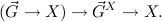
In our implementation this function is called
| (atr-goals-to-x-proof goal1 ...) |
 and goal formulas
  we can derive in minimal
logic
we can derive in minimal
logic
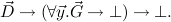
Then we can also derive in intuitionistic logic augmented with the special predicate variable X
In particular, substitution of the formula
for X yields a derivation in intuitionistic logic of

This is done by
| (atr-min-excl-proof-to-x-proof min-excl-proof) | |||||
| (atr-min-excl-proof-to-intuit-ex-proof min-excl-proof) |
S:ExtrTerms
| (formula-to-et-type formula) |
When we want to execute the program, we have to replace the constant cL corresponding to a lemma L by the extracted program of its proof, and the constant cGA corresponding to a global assumption GA by an assumed extracted term to be provided by the user. This can be achieved by adding computation rules for cL and cGA. We can be rather flexible here and enable/block rewriting by using animate/deanimate as desired. Notice that the type of the extracted term provided for a cGA must be the extracted type of the assumed formula. When predicate variables are present, one must use the type variables assigned to them in PVAR-TO-TVAR-ALIST.
| (animate thm-or-ga-name . opt-eterm) | |||||
| (deanimate thm-or-ga-name) |
We can define, for a given derivation M of a formula A with τ(A) nulltype,
its extracted term (or extracted program) et(M) of type τ(A). We also need
extracted terms for the axioms. For induction we take recursion, for the
proof-by-cases axiom we take the cases-construct for terms; for the other axioms
the extracted terms are rather clear. Term extraction is implemented
by
nulltype,
its extracted term (or extracted program) et(M) of type τ(A). We also need
extracted terms for the axioms. For induction we take recursion, for the
proof-by-cases axiom we take the cases-construct for terms; for the other axioms
the extracted terms are rather clear. Term extraction is implemented
by
| (proof-to-extracted-term proof) |
It is also possible to give an internal proof of soundness. This can be done by
| (proof-to-soundness-proof proof) |
Reading
| (py string) | for parsing types | ||||||
| (pv string) | for parsing variables | ||||||
| (pt string) | for parsing terms | ||||||
| (pf string) | for parsing formulas |
The conversion occurs in two steps: lexical analysis and parsing.
14.1. Lexical analysis. In this stage the string is brocken into short sequences, called tokens.
A token can be one of the following:
For example: abc, ABC and A are alphabetic symbols, 123, 0123 and 7 are numbers, ( is a punctuation mark, and <=, +, and #:-ˆ are special symbols.
Tokens are always character sequences of maximal length belonging to one of the above categories. Therefore fx is a single alphabetic symbol not two and likewise <+ is a single special symbol. The sequence alpha<=(-x+z), however, consists of the 8 tokens alpha, <=, (, -, x, +, z, and ). Note that the special symbols <= and - are separated by a punctuation mark, and the alphabetic symbols x and z are separated by the special symbol +.
If two alphabetic symbols, two special symbols, or two numbers follow each other they need to be separated by white space (spaces, newlines, tabs, formfeeds, etc.). Except for a few situations mentioned below, whitespace has no significance other than separating tokens. It can be inserted and removed between any two tokens without affecting the significance of the string.
Every token has a token type, and a value. The token type is one of the following: number, var-index, var-name, const, pvar-name, predconst, type-symbol, pscheme-symbol, postfix-op, prefix-op, binding-op, add-op, mul-op, rel-op, and-op, or-op, imp-op, pair-op, if-op, postfix-jct, prefix-jct, and-jct, or-jct, tensor-jct, imp-jct, quantor, dot, hat, underscore, comma, semicolon, arrow, lpar, rpar, lbracket, rbracket.
The possible values for a token depend on the token type and are explained below.
New tokens can be added using the function

The inverse is the function

A list of all currently defined tokens sorted by token types can be obtained by the function
14.2. Parsing. The second stage, parsing, extracts structure form the sequence of tokens.
Types. Type-symbols are types; the value of a type-symbol must be a type. If σ and τ are types, then σ;τ is a type (pair type) and σ=>τ is a type (function type). Parentheses can be used to indicate proper nesting. For example boole is a predefined type-symbol and hence, (boole;boole)=>boole is again a type. The parentheses in this case are not strictly necessary, since ; binds stronger than =>. Both operators associate to the right.
Variables. Var-names are variables; the value of a var-name token must be a pair consisting of the type and the name of the variable (the same name string again! This is not nice and may be later, we find a way to give the parser access to the string that is already implicit in the token). For example to add a new boolean variable called “flag”, you have to invoke the function (add-token "flag" ’var-name (cons ’boole "flag")). This will enable the parser to recognize “flag3”, “flagˆ”, or “flagˆ14” as well.
Further, types, as defined above, can be used to construct variables.
A variable given by a name or a type can be further modified. If it is followed by a ˆ, a partial variable is constructed. Instead of the ˆ a _ can be used to specify a total variable.
Total variables are the default and therefore, the _ can be omitted.
As another modifier, a number can immediately follow, with no whitespace in between, the ˆ or the _, specifying a specific variable index.
In the case of indexed total variables given by a variable name or a type symbol, again the _ can be omitted. The number must then follow, with no whitespace in between, directly after the variable name or the type.
Note: This is the only place where whitespace is of any significance in the input. If the ˆ, _, type name or variable name is separated from the following number by whitespace, this number is no longer considered to be an index for that variable but a numeric term in its own right.
For example, assuming that p is declared as a variable of type boole, we have:
Terms are built from atomic terms using application and operators.
An atomic term is one of the following: a constant, a variable, a number, a conditional, or any other term enclosed in parentheses.
Constants have const as token type, and the respective term in internal form as value. There are also composed constants, so-called constant schemata. A constant schema has the form of the name of the constant schema (token type constscheme) followed by a list of types, the whole thing enclosed in parentheses. There are a few built in constant schemata: (Rec <typelist>) is the recursion over the types given in the type list; (EQat <type>) is the equality for the given type; (Eat <type>) is the existence predicate for the given type. The constant schema EQat can also be written as the relational infix operator =; the constant schemata Eat can also be written as the prefix operator E.
For a number, the user defined function make-numeric-term is called with the number as argument. The return value of make-numeric-term should be the internal term representation of the number.
To form a conditional term, the if operator if followed by a list of atomic terms is enclosed in square brackets. Depending on the constructor of the first term, the selector, a conditional term can be reduced to one of the remaining terms.
From these atomic terms, compound terms are built not only by application but also using a variety of operators, that differ in binding strength and associativity.
Postfix operators (token type postfix-op) bind strongest, next in binding strength are prefix operators (token type prefix-op), next come binding operators (token type binding-op).
A binding operator is followed by a list of variables and finally a term. There are two more variations of binding operators, that bind much weaker and are discussed later.
Next, after the binding operators, is plain application. Juxtaposition of two terms means applying the first term to the second. Sequences of applications associate to the left. According to the vector notation convention the meaning of application depends on the type of the first term. Two forms of applications are defined by default: if the type of the first term is of arrow-form? then make-term-in-app-form is used; for the type of a free algebra we use the corresponding form of recursion. However, there is one exception: if the first term is of type boole application is read as a short-hand for the “if...then ...else” construct (which is a special form) rather than boolean recursion. The user may use the function add-new-application to add new forms of applications. This function takes two arguments, a predicate for the type of the first argument, and a function taking the two terms and returning another term intended to be the result of this form of application. Predicates are tested in the inverse order of their definition, so more general forms of applications should be added first.
By default these new forms of application are not used for output; but the user might declare that certain terms should be output as formal application. When doing so it is the user’s responisbility to make sure that the syntax used for the output can still be parsed correctly by the parser! To do so the function (add-new-application-syntax pred toarg toop) can be used, where the first argument has to be a predicate (i.e., a function mapping terms to #t and #f) telling whether this special form of application can be used. If so, the arguments toarg and toop have to be functions mapping the term to operator and argument of this “application” respectively.
After that, we have binary operators written in infix notation. In order of decreasing binding strength these are:
On the top level, we have two more forms of binding operators, one using the dot “.”, the other using square brackets “[ ]”. Recall that a binding operator is followed by a list of variables and a term. This notation can be augmented by a period “.” following after the variable list and before the term. In this case the scope of the binding extends as far to the right as possible. Bindings with the lambda operator can also be specified by including the list of variables in square brackets. In this case, again, the scope of the binding extends as far as possible.
Predefined operators are E and = as described above, the binding operator lambda, and the pairing operator @ with two prefix operators left and right for projection.
The value of an operator token is a function that will obtain the internal representation of the component terms as arguments and returns the internal representation of the whole term.
If a term is formed by application, the function make-gen-application is called with two subterms and returns the compound term. The default here (for terms with an arrow type) is to make a term in application form. However other rules of composition might be introduced easily.
Formulas are built from atomic formulas using junctors and quantors.
The simplest atomic formulas are made from terms using the implicit predicate “atom”. The semantics of this predicate is well defined only for terms of type boole. Further, a predicate constant (token type predconst) or a predicate variable (token type pvar) followed by a list of atomic terms is an atomic formula. Lastly, any formula enclosed in parentheses is considered an atomic formula.
The composition of formulas using junctors and quantors is very similar to the composition of terms using operators and binding. So, first postfix junctors, token type postfix-jct, are applied, next prefix junctors, token type prefix-jct, and quantors, token type quantor, in the usual form: quantor, list of variables, formula. Again, we have a notation using a period after the list of variables, making the scope of the quantor as large as possible. Predefined quantors are ex, excl, exca, and all.
The remaining junctors are binary junctors written in infix form. In order of decreasing binding strength we have:
Predefined junctors are & (and), ! (tensor), and -> (implication).
The value of junctors and quantors is a function that will be called with the appropriate subformulas, respectively variable lists, to produce the compound formula in internal form.
[1] Klaus Aehlig and Helmut Schwichtenberg, A syntactical analysis of non-size-increasing polynomial time computation, Proceedings 15’th Symposium on Logic in Computer Science (LICS 2000), 2000, pp. 84–91.
[2] Ulrich Berger, Program extraction from normalization proofs, Typed Lambda Calculi and Applications (M. Bezem and J.F. Groote, eds.), LNCS, vol. 664, Springer Verlag, Berlin, Heidelberg, New York, 1993, pp. 91–106.
[3] Ulrich Berger, Wilfried Buchholz, and Helmut Schwichtenberg, Refined program extraction from classical proofs, Annals of Pure and Applied Logic 114 (2002), 3–25.
[4] Ulrich Berger, Matthias Eberl, and Helmut Schwichtenberg, Term rewriting for normalization by evaluation, Information and Computation 183 (2003), 19–42.
[5] Ulrich Berger and Helmut Schwichtenberg, An inverse of the evaluation functional for typed λ-calculus, Proceedings 6’th Symposium on Logic in Computer Science (LICS’91) (R. Vemuri, ed.), IEEE Computer Society Press, Los Alamitos, 1991, pp. 203–211.
[6] Stefan Berghofer, Proofs, programs and executable specifications in higher order logic, Ph.D. thesis, Institut für Informatik, TU München, 2003.
[7] Martin Hofmann, Linear types and non-size-increasing polynomial time computation, Proceedings 14’th Symposium on Logic in Computer Science (LICS’99), 1999, pp. 464–473.
[8] Felix Joachimski and Ralph Matthes, Short proofs of normalisation for the simply-typed λ-calculus, permutative conversions and Gödel’s T, Archive for Mathematical Logic 42 (2003), 59–87.
[9] Ralph Matthes, Extensions of System F by Iteration and Primitive Recursion on Monotone Inductive Types, Ph.D. thesis, Mathematisches Institut der Universität München, 1998.
[10] Dale Miller, A logic programming language with lambda–abstraction, function variables and simple unification, Journal of Logic and Computation 2 (1991), no. 4, 497–536.
[11] Tobias Nipkow, Higher-order critical pairs, Proceedings of the Sixth Annual IEEE Symposium on Logic in Computer Science (Los Alamitos) (R. Vemuri, ed.), IEEE Computer Society Press, 1991, pp. 342–349.
[12] Viggo Stoltenberg-Hansen, Edward Griffor, and Ingrid Lindström, Mathematical theory of domains, Cambridge Tracts in Theoretical Computer Science, Cambridge University Press, 1994.
[13] Anne S. Troelstra and Helmut Schwichtenberg, Basic proof theory, 2nd ed., Cambridge University Press, 2000.
=-to-E-1, 1
=-to-E-2, 2
=-to-Eq, 3
aconst-to-formula, 4
aconst-to-inst-formula, 5
aconst-to-kind, 6
aconst-to-name, 7
aconst-to-repro-formulas, 8
aconst-to-string, 9
aconst-to-tpsubst, 10
aconst-to-uninst-formula, 11
aconst-without-rules?, 12
aconst=?, 13
add-alg, 16
add-algebras-with-parameters, 17
add-algs, 18
add-computation-rule, 19
add-global-assumption, 20
add-ids, 21
add-new-application, 22
add-param-alg, 23
add-param-algs, 24
add-predconst-name, 25
add-program-constant, 26
add-pvar-name, 27
add-rewrite-rule, 28
add-theorem, 29
add-tvar-name, 30
add-var-name, 31
aga, 32
alg-form-to-name, 33
alg-form-to-types, 34
alg-form?, 35
alg-name-to-arity, 36
alg-name-to-simalg-names, 37
alg-name-to-token-types, 38
alg-name-to-tvars, 39
alg-name-to-typed-constr-names, 40
alg?, 41
all-allpartial-aconst, 45
All-AllPartial-nat, 46
all-form-to-kernel, 47
all-form-to-var, 48
all-form-to-vars-and..., 49
all-form?, 50
all-formula-to-cases-aconst, 51
all-formulas-to-ind-aconst, 52
allnc-form-to-kernel, 53
allnc-form-to-var, 54
allnc-form?, 55
allpartial-all-aconst, 58
AllPartial-All-nat,, 59
and-form-to-left, 60
and-form-to-right, 61
and-form?, 62
animate, 63
animation, 64
arity
of a predicate variable, 65
of a program constant, 66
arity-to-string, 67
arity-to-types, 68
arrow-form-to-arg-type, 69
arrow-form-to-arg-types, 70
arrow-form-to-final-val-type, 71
arrow-form-to-val-type, 72
arrow-form?, 73
arrow-types-to-rec-const, 74
assume, 75
assumption constant, 76
asubst, 77
Atom-False, 78
atom-form-to-kernel, 79
atom-form?, 80
Atom-True, 81
atr-arb-definite-proof, 82
atr-arb-goal-proof, 83
atr-definite?, 84
atr-goal?, 85
atr-goals-to-x-proof, 86
atr-irrel-goal-proof, 87
atr-min-...-to-intuit-ex-proof, 88
atr-min-excl-proof-to-x-proof, 89
atr-rel-definite-proof, 90
atr-relevant?, 91
avar-proof-equal?, 92
avar-to-formula, 93
avar-to-index, 94
avar-to-name, 95
avar=?, 96
avar=?, 97
avar?, 98
Berger, 99
bottom, 100
by-assume-with, 101
by-exnc-assume-with, 102
cases, 105
cases-construct, 106
Cases-Log, 107
check-and-display-proof, 108
classical-cterm=?, 109
clause, 112
Compatibility, 113
Compose, 114
compose-o-substitutions, 115
compose-substitutions, 116
compose-substitutions-wrt, 117
compose-t-substitutions, 118
composition, 119
computation rule, 122
computation rules, 123
consistent-substitutions-wrt?, 124
const-to-arrow-types-or..., 125
const-to-kind, 126
const-to-name, 127
const-to-object-or-arity, 128
const-to-t-deg, 129
const-to-token-type, 130
const-to-tsubst, 131
const-to-tvars, 132
const-to-type, 133
const-to-uninst-type, 134
const=?, 135
const?, 136
constant scheme, 137
constr-name-and-tsubst..., 138
constr-name-to-constr, 139
constr-name?, 140
Constr-Total, 141
Constr-Total-Args, 142
constructor, 143
constructor pattern, 144
context, 145
context-to-avars, 146
context-to-vars, 147
context=?, 148
conversion relation, 149
Coquand, 150
cterm-subst, 151
cterm-substitute, 152
cterm-to-formula, 153
cterm-to-free, 154
cterm-to-string, 155
cterm-to-vars, 156
cterm=?, 157
cterm?, 158
current-goal, 159
current-proof, 160
cut, 161
Cvind-with-measure-11, 162
deanimate, 163
degree of totality, 166
display-constructors, 167
display-current-goal, 168
display-current-goal-with..., 169
display-current-num-goals..., 170
display-global-assumptions, 171
display-normalized-proof, 172
display-normalized-proof-expr, 173
display-normalized-pterm, 174
display-p-substitution, 175
display-program-constants, 176
display-proof, 177
display-proof-expr, 178
display-pterm, 179
display-substitution, 180
display-t-substitution, 181
display-theorems, 182
dnp, 183
dnpe, 184
dnpt, 185
cdp, 186
dp, 187
dpe, 188
dpt, 189
drop, 190
E, 191
E-to-Total, 192
E-to-Total-nat, 193
Efq, 194
Efq-Atom, 195
Efq-Log, 196
Elim, 197
elim, 198
empty-subst, 199
Eq, 200
Eq-Compat, 201
eq-compat-aconst, 202
Eq-Ext, 203
eq-refl-aconst, 206
eq-symm-aconst, 209
Eq-to-=-1, 210
Eq-to-=-1-nat, 211
Eq-to-=-2, 212
Eq-to-=-2-nat, 213
eq-trans-aconst, 216
equal-pvars?, 217
=-Refl-nat, 218
=-Symm-nat, 219
=-Trans-nat, 220
equality, 221
=-to-E-1-nat, 222
=-to-E-2-nat, 223
=-to-Eq-nat, 224
evaluation, 225
Ex-Elim, 229
ex-elim, 230
ex-expartial-aconst, 233
Ex-ExPartial-nat, 234
ex-form-to-kernel, 235
ex-form-to-var, 236
ex-form-to-vars-and..., 237
ex-form?, 238
ex-for...-to-ex-elim-const, 239, 240
ex-formula-to-ex-intro-aconst, 241
Ex-Intro, 244
ex-intro, 245
exc-elim, 246
exc-intro, 247
exca, 248
exca-form-to-kernel, 249
exca-form-to-var, 250
exca-form?, 251
excl, 252
excl-form-to-kernel, 253
excl-form-to-var, 254
excl-form?, 255
exnc-elim, 256
exnc-form-to-kernel, 257
exnc-form-to-var, 258
exnc-form?, 259
exnc-intro, 260
expand-theorems, 261
expartial-ex-aconst, 265
ExPartial-Ex-nat, 266
ext-aconst, 267
Extensionality, 268
extracted program, 269
extracted term, 270
falsity, 271
falsity-log, 272
Filliatre, 273
finalg-to-=-const, 274
finalg-to-=-to-e-1-aconst, 275
finalg-to-=-to-e-2-aconst, 276
finalg-to-=-to-eq-aconst, 277
finalg-to-all-allpartial-aconst, 278
finalg-to-e-const, 279
finalg-to-e-to-total-aconst, 280
finalg-to-eq-to-=-1-aconst, 281
finalg-to-eq-to-=-2-aconst, 282
finalg-to-expartial-ex-aconst, 283
finalg-to-total-to-e-aconst, 284
finalg?, 285
fold-cterm, 286
fold-formula, 287
formula
definite, 288
folded, 289
goal, 290
prime, 291
relevant, 292
unfolded, 293
formula-subst, 294
formula-substitute, 295
formula-to-et-type, 296
formula-to-free, 297
formula-to-prime-subformulas, 298
formula-to-string, 299
get, 302
global assumption, 303
global-assdots-name-to-aconst, 304
goal, 305
goal-subst, 306
goal-to-context, 307
goal-to-formula, 308
goal-to-goalvar, 309
goal=?, 310
ground-type?, 311
Harrop degree, 312
Harrop formula, 313
Huet, 314
imp-form-to-conclusion, 317
imp-form-to-final-conclusion, 318
imp-form-to-premise, 319
imp-form-to-premises, 320
imp-form?, 321
imp-formulas-to-elim-aconst, 322
Ind, 325
ind, 326
induction, 327
inst-with, 328
inst-with-to, 329
Intro, 330
intro, 331
intro-search, 332
Letouzey, 333
lexical analysis, 334
make-=, 335
make-aconst, 336
make-alg, 337
make-all, 338
make-allnc, 339
make-and, 340
make-arity, 341
make-arrow, 342
make-atomic-formula, 343
make-avar, 344
make-const, 345
make-cterm, 346
make-e, 347
make-eq, 348
make-ex, 349
make-exca, 350
make-excl, 351
make-exnc, 352
make-imp, 353
make-inhabited, 354
make-predconst, 355
make-predicate-formula, 356
make-proof-in-aconst-form, 357
make-proof-in-all-elim-form, 358
make-proof-in-all-intro-form, 359
make-proof-in-and-elim-l..., 360
make-proof-in-and-elim-r..., 361
make-proof-in-and-intro-form, 362
make-proof-in-avar-form, 363
make-proof-in-cases-form, 364
make-proof-in-ex-intro-form, 365
make-proof-in-imp-elim-form, 366
make-proof-in-imp-intro-form, 367
make-pvar, 368
make-quant-formula, 369
make-star, 370
make-subst, 371
make-subst-wrt, 372
make-substitution, 373
make-substitution-wrt, 374
make-tensor, 375
make-term-in-abst-form, 376
make-term-in-app-form, 377
make-term-in-const-form, 378
make-term-in-if-form, 379
make-term-in-lcomp-form, 380
make-term-in-pair-form, 381
make-term-in-rcomp-form, 382
make-term-in-var-form, 383
make-total, 384
min-pr, 387
Minpr-with-measure-l11, 388
mk-all, 389
mk-allnc, 390
mk-and, 391
mk-arrow, 392
mk-ex, 393
mk-exca, 394
mk-excl, 395
mk-exnc, 396
mk-imp, 397
mk-neg, 398
mk-neg-log, 399
mk-proof-in-and-intro-form, 400
mk-proof-in-elim-form, 401
mk-proof-in-ex-intro-form, 402
mk-proof-in-intro-form, 403
mk-quant, 404
mk-tensor, 405
mk-term-in-abst-form, 406
mk-term-in-app-form, 407
mk-var, 408
name-hyp, 409
nbe-constr-value-to-constr, 410
nbe-constr-value-to-name, 411
nbe-constr-value?, 412
nbe-constructor-pattern?, 413
nbe-extract, 414
nbe-fam-value?, 415
nbe-formula-to-type, 416
nbe-genargs, 417
nbe-inst?, 418
nbe-make-constr-value, 419
nbe-make-object, 420
nbe-match, 421
nbe-normalize-proof, 422
nbe-normalize-term, 423
nbe-object-app, 424
nbe-object-apply, 425
nbe-object-compose, 426
nbe-object-to-type, 427
nbe-object-to-value, 428
nbe-object?, 429
nbe-pconst-...-to-object, 430
nbe-reflect, 431
nbe-reify, 432
nbe-term-to-object, 433
new-tvar, 434
nf, 435
ng, 436
Nipkow, 437
normalize-formula, 438
normalize-goal, 439
np, 440
nf, 441
nt, 442
number-and-idpredconst-to-intro-aconst, 443
numerated-var-to-index, 444
numerated-var, 445
object-type?, 446
osubst, 447
p-substitution-to-string, 448
pair-elim, 449
parsing, 450
pattern-unify, 451
Paulin-Mohring, 452
Paulson, 453
pconst-name-to-comprules, 454
pconst-name-to-inst-objs, 455
pconst-name-to-object, 456
pconst-name-to-pconst, 457
pconst-name-to-rewrules, 458
pf, 459
pproof-state-to-formula, 460
pproof-state-to-proof, 461
predconst-name-to-arity, 462
predconst-name?, 463
predconst-to-index, 464
predconst-to-name, 465
predconst-to-string, 466
predconst-to-tsubst, 467
predconst-to-uninst-arity, 468
predconst?, 469
predicate constant, 470
predicate-form-to-args, 471
predicate-form-to-predicate, 472
predicate-form?, 473
prename, 474
Presburger, 475
prime-form?, 476
proof-in-aconst-form-to-aconst, 477
proof-in-aconst-form?, 478
proof-in-all-elim-form-to-arg, 479
proof-in-all-elim-form-to-op, 480
proof-in-all-elim-form?, 481
pr...all-intro-form-to-kernel, 482
pr...all-intro-form-to-var, 483
proof-in-all-intro-form?, 484
proof-in-and-elim..., 485
proof-in-and-elim-left-form?, 486
proof-in-and-elim..., 487
proof-in-and-elim-right-form?, 488
pr...and-intro-form-to-left, 489
pr...and-intro-form-to-right, 490
proof-in-and-intro-form?, 491
proof-in-avar-form-to-avar, 492
proof-in-avar-form?, 493
proof-in-cases-form-to-alts, 494
proof-in-cases-form-to-rest, 495
proof-in-cases-form-to-test, 496
proof-in-cases-form?, 497
proof-in-elim-form-to-args, 498
pr...elim-form-to-final-op, 499
proof-in-imp-elim-form-to-arg, 500
proof-in-imp-elim-form-to-op, 501
proof-in-imp-elim-form?, 502
proof-in-imp-intro-form-to-avar, 503
pr...-imp-intro-form-to-kernel, 504
proof-in-imp-intro-form?, 505
proof-in-intro-form-to..., 506
proof-of-efq-at, 507
proof-of-efq-log-at, 508
proof-of-stab-at, 509
proof-of-stab-log-at, 510
proof-subst, 511
proof-substitute, 512
proof-to-aconsts, 513
proof-to-aconsts-without-rules, 514
proof-to-bound-avars, 515
proof-to-context, 516
proof-to-expr, 517
proof-to-extracted-term, 518
proof-to-formula, 519
proof-to-free, 520
proof-to-free-and-bound-avars, 521
proof-to-free-avars, 522
proof-to-soundness-proof, 523
proof=?, 524
proof?, 525
proofs=?, 526
psubst, 527
pt, 528
pv, 529
pvar-cterm-equal?, 530
pvar-name-to-arity, 531
pvar-name?, 532
pvar-to-arity, 533
pvar-to-h-deg, 534
pvar-to-index, 535
pvar-to-name, 536
pvar?, 537
py, 538
Q-clause, 539
Q-sequent, 542
Q-substitution, 543
Q-term, 544
quant-form-to-kernel, 545
quant-form-to-quant, 546
quant-form-to-vars, 547
quant-form?, 548
quant-free?, 549
quant-prime-form?, 550
Rec, 551
Rec, 552
recursion, 553
recursion operator, 554
reduce-efq-and-stab, 555
remove-alg-name, 556
remove-computation-rules-for, 557
remove-global-assumption, 558
remove-predconst-name, 559
remove-program-constant, 560
remove-pvar-name, 561
remove-rewrite-rules-for, 562
remove-theorem, 563
remove-tvar-name, 564
remove-var-name, 565
rename, 566
restrict-substitution-to-args, 567
restrict-substitution-wrt, 568
rewrite rule, 569
rm-exc, 570
save, 571
search, 572
select, 573
semantical model, 574
set-goal, 575
simind, 576
simp, 577
simp-with, 578
special form, 579
split, 580
Stab, 581
Stab-Atom, 582
Stab-Log, 583
star-form-to-left-type, 584
star-form-to-right-type, 585
star-form?, 586
strip, 587
strong elimination, 588
subst-item-equal-wrt?, 589
substitution-equal-wrt?, 590
substitution-equal?, 591
substitution-to-string, 592
synt-total?, 593
tensor-form-to-left, 594
tensor-form-to-parts, 595
tensor-form-to-right, 596
tensor-form?, 597
term-in-abst-form-to-kernel, 598
term-in-abst-form-to-var, 599
term-in-abst-form?, 600
term-in-app-form-to-arg, 601
term-in-app-form-to-args, 602
term-in-app-form-to-final-op, 603
term-in-app-form-to-op, 604
term-in-app-form?, 605
term-in-const-form-to-const, 606
term-in-const-form?, 607
term-in-if-form-to-alts, 608
term-in-if-form-to-rest, 609
term-in-if-form-to-test, 610
term-in-if-form?, 611
term-in-lcomp-form-to-kernel, 612
term-in-lcomp-form?, 613
term-in-pair-form-to-left, 614
term-in-pair-form-to-right, 615
term-in-pair-form?, 616
term-in-rcomp-form-to-kernel, 617
term-in-rcomp-form?, 618
term-in-var-form-to-var, 619
term-in-var-form?, 620
term-subst, 621
term-substitute, 622
term-to-bound, 623
term-to-free, 624
term-to-string, 625
term-to-t-deg, 626
term-to-type, 627
term=?, 628
term?, 629
terms=?, 630
theorem-name-to-aconst, 631, 632
theorem-name-to-inst-proof, 633
theorem-name-to-proof, 634
token, 635
total-aconst, 640
Total-to-E, 641
Total-to-E-nat, 642
truth, 643
truth-aconst, 644
tsubst, 647
tvar-to-index, 648
tvar-to-name, 649
tvar?, 650
type constant, 651
type substitutions, 652
type variable, 653
type-subst, 654
type-substitute, 655
type-to-new-partial-var, 656
type-to-new-var, 657
type-to-string, 658
type?, 659
undo, 660
unfold-cterm, 661
unfold-formula, 662
use, 663
use-with, 664
var-form?, 665
var-term-equal?, 666
var-to-index, 667
var-to-name, 668
var-to-new-var, 669
var-to-t-deg, 670
var-to-type, 671
var?, 672
vector notation, 673
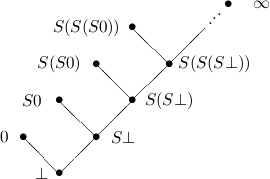


 (
(
 (
(
 )
) 
 )
) 
 )
) )
) 


 )
)  )
) )
)  )
) (
(
 )
)  (
( )
)
 )
)  (
( ))
))  (
( (
(
 )
)  (
( )
)
 )
)  (
( ))
))  (
( (
(
 )
)  (
( )
)
 )
)  (
( ))
))  (
(


 (
( (
(
 (
(


 (
( (
( (
(


