3. First steps: Linear Classification¶

Two traditional machine learning models for linear classifications are:

The Perceptron and
The Adaptive Linear Neuron.

The ideas for these two models go back to

McCulloh & Pitts (1943) [mcculloch_logical_1943]
Rosenblatt (1957) [rosenblatt_perceptron_1957]
Widrow (1960) [widrow_adapting_1960]

These models provide a good entry point also for modern machine learning algorithms as:

They are very simple;
but also generalizes to the modern deep networks.

This section is inspired by the introductory chapters of the book [raschka_python_2015].

3.1. Binary Classification Problems¶

As an example of a typical of a binary classification problem let us consider:

A sequence of \(N\) data points \(x^{(i)}\in\mathbb R^n, 1\leq i\leq N\);
each having \(n\) characteristic features \(x^{(i)}=(x^{(i)}_1,x^{(i)}_2,\ldots,x^{(i)}_n)\);
and the task to assign to each element \(x^{(i)}\) a label \(y^{(i)}\in\{-1,+1\}\);
thereby dividing the data points into two classes labeled \(-1\) and \(+1\).

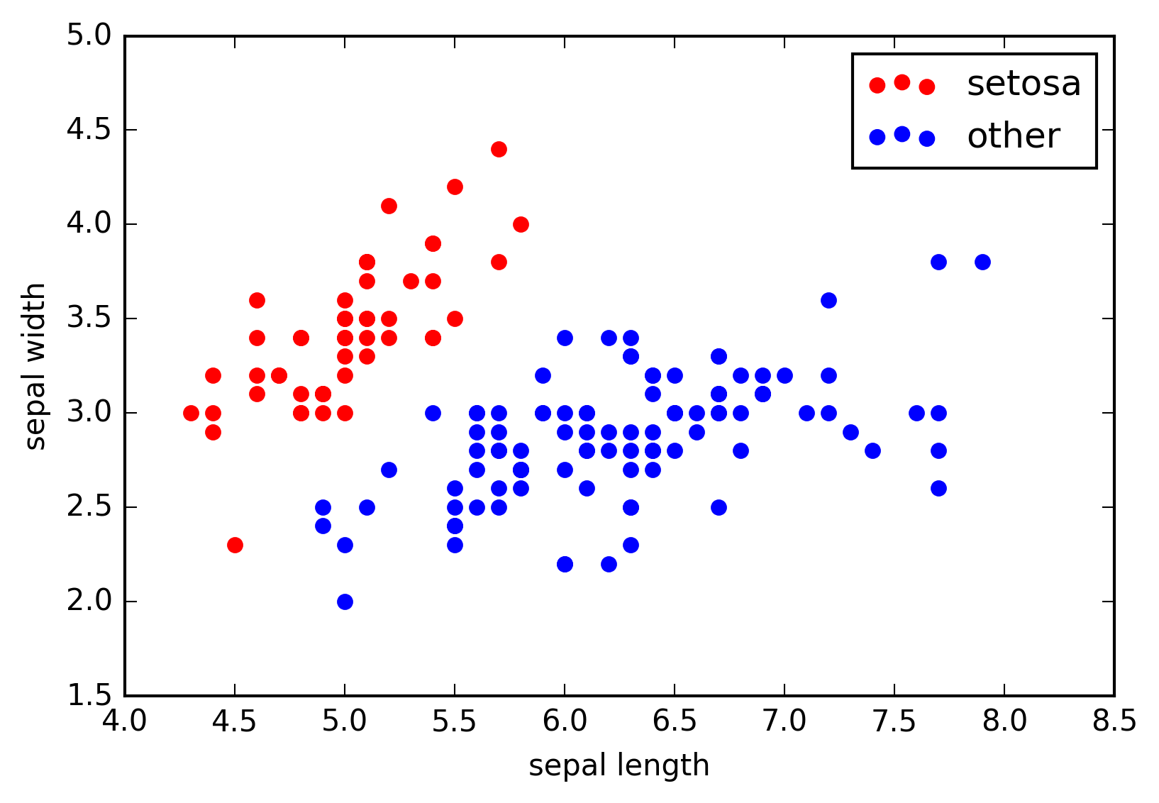
Labelled 2d example data points (\(x^{(i)}\in\mathbb R^2\)) describing the sepal length and width (\(x^{(i)}_1\) and \(x^{(i)}_2\), respectively) of species of the iris flower. The respected class labels ‘setosa’ and ‘other’, i.e., \(y^{(i)}\in\{-1,+1\}\), are encoded in the colors red and blue.

The goal of the classification problem is, given some pre-labeled training data:

\[(x^{(i)},y^{(i)})_{1\leq i\leq M}, \qquad M\leq N\]

to find a function

\[f:\mathbb R^n \to \{-1,+1\}\]

that:

predicts accurately the labels of pre-labeled training data \((x^{(i)},y^{(i)})_{1\leq i\leq M}\), i.e., for most indices \(i\in\{1,\ldots,M\}\) it should hold \(f(x^{(i)})=y^{(i)}\);
and generalizes well to unknown data.

A general approach to this problem is to specify a space of candidates for \(f\), the hypothesis set. Then the art of the game is to find sensible mathematical counterparts for the vague terms ‘accurately’ and ‘generalizes’ and to find, in that sense, optimal functions \(f\).

Typically one tries to find an appropriate parametrization of the hypothesis set, so that the search for an optimal \(f\) can then be recast into a search for optimal parameters;
In which sense parameters are better or worse than others is usually encoded by a real-valued function on this parameter space which depends on the training data, often called ‘loss’, ‘regret’, ‘energy’ or ‘error’ function;
The search for optimal parameters is then recast into a search of minima of this loss function.

One calls the classification problem linear if the data points of the two classes can be separated by a hyperplane.

The following plot shows the data points of the iris data set shown above with a possible hyperplane as decision boundary between the two different classes.

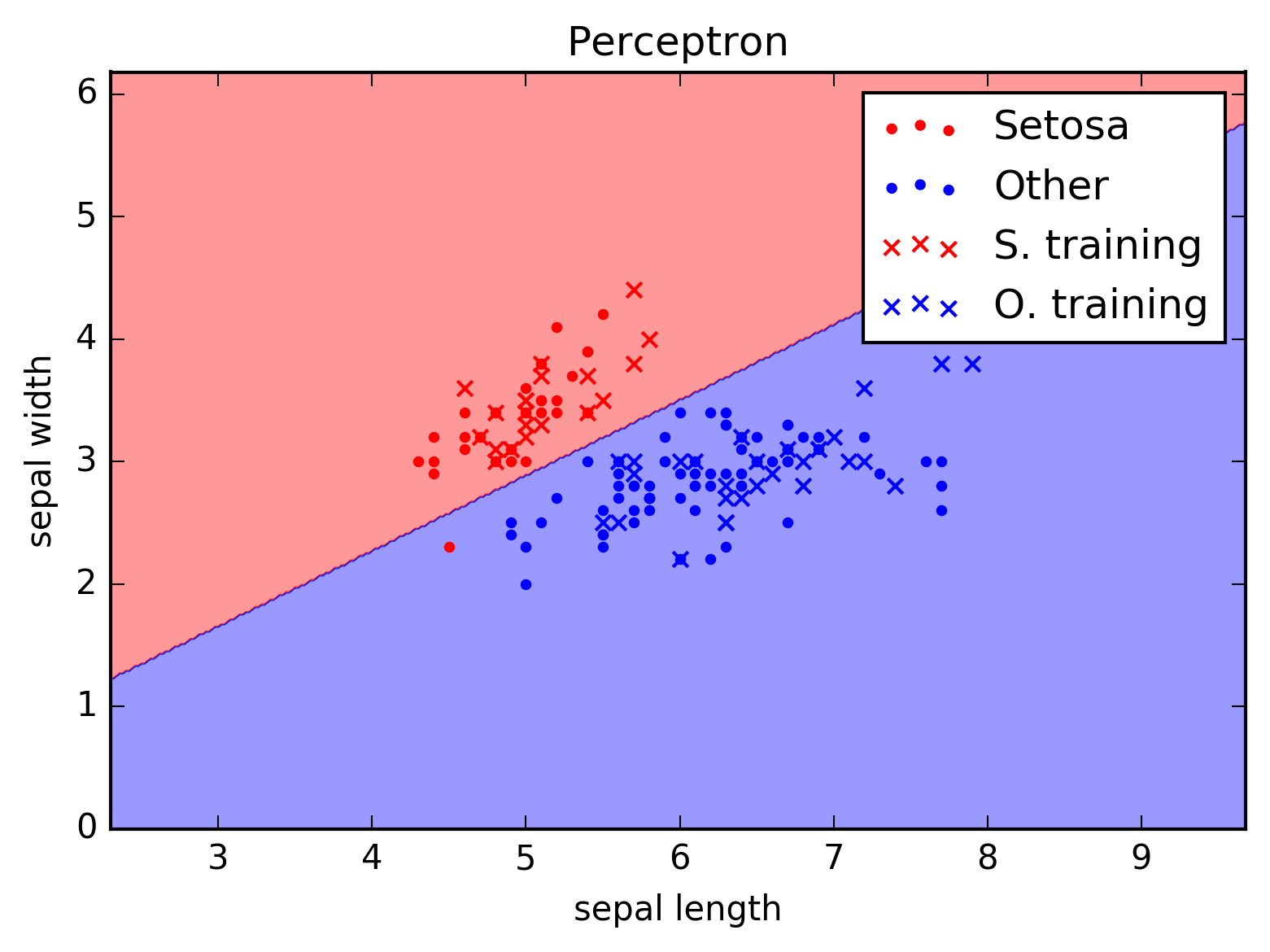
_images/linear_classification_decission.png

Decission boundaries for a possible classification function \(f\). The dots denote unknown data points and the crosses denote pre-labeled data points which were used to train the machine learning model in order to find an optimal \(f\).

Note that although the classification of the pre-labeled data points (the crosses) seems to be perfect, the classification of the unknown data (points) is not. This may be due to the fact that either:

the data is simply not separable using just a hyperplane, in which case one calls the problem ‘non-linear classification problem’,
or there are errors in the pre-labeled data.

It is quite a typical situation that a perfect classification is not possible. It is therefore important to specify mathematically in which sense we allow for errors and what can be done to minimize them – this will be encoded in the mathematical sense given to ‘accurately’ and ‘generalizes’, i.e., in terms of the loss function, as discussed above.

In the following we will specify two senses which lead to the model of the Perceptron and Adaline.

3.2. Perceptron¶

The first model we will take a look is the so-called Perceptron model. It is a mathematical model inspired by a nerve cell:

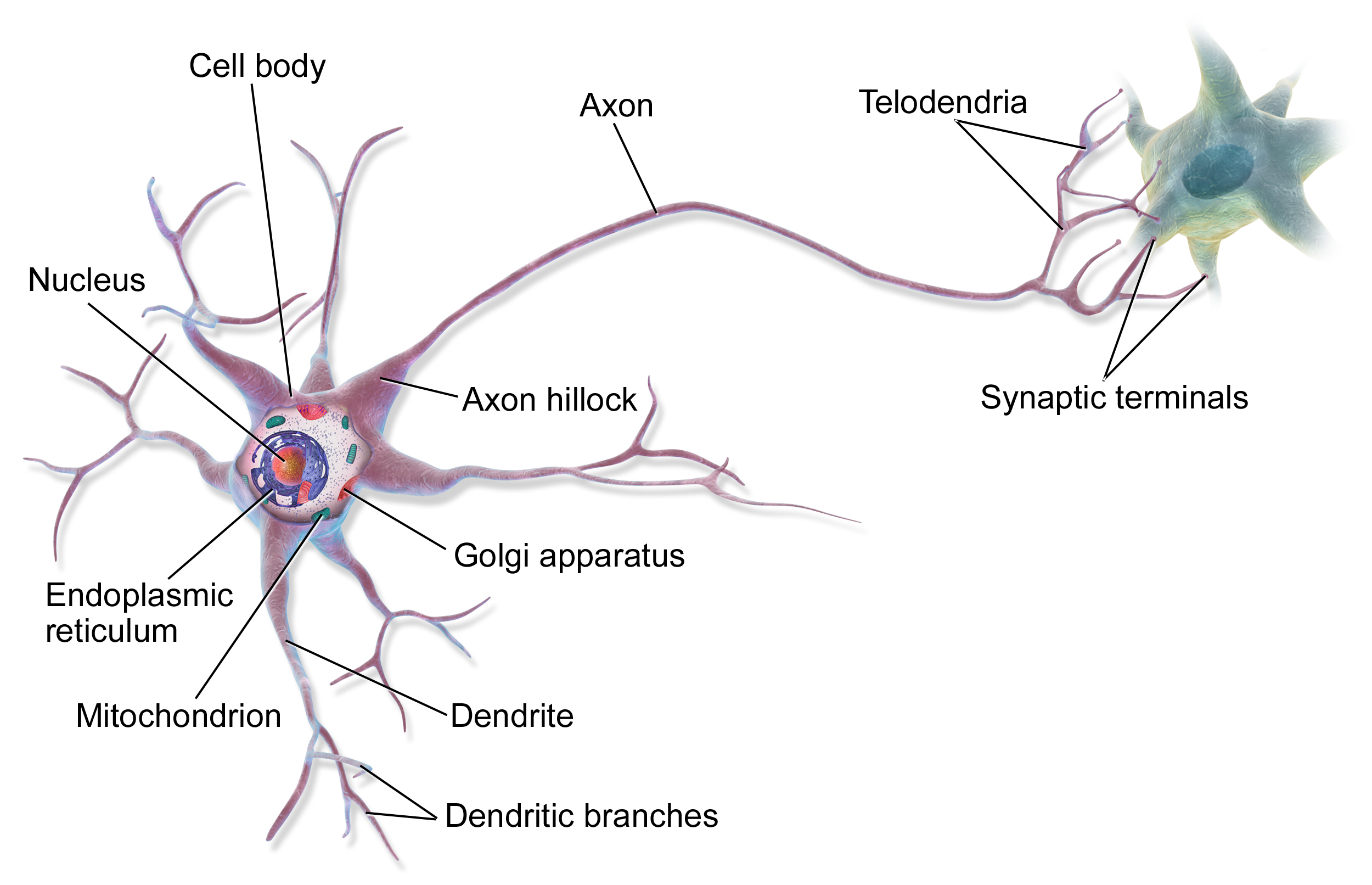
A sketch of a neuron (source).

The mathematical model can be sketched as follows:

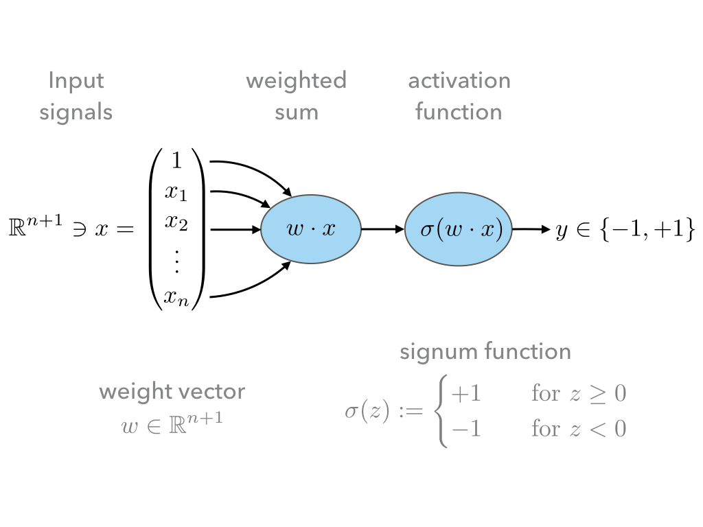
The input signals are given as a vector \(x\in\mathbb R^{n+1}\);
These input signals are weighted by the weight vector \(w\in\mathbb R^{n+1}\),
and then summed to give \(w\cdot x\).
The first coefficient in the input vector \(x\) is always assumed to be one, and thus, the first coefficient in the weight vector \(w\) is a threshold term, which renders \(w\cdot x\) an affine linear as opposed to a just linear map.
Finally signum function is employed to infer from \(w\cdot x\in\mathbb R\) discrete class labels \(y\in\{-1,+1\}\).

This results in a hypothesis set of function \(f_w\)

(1)¶\[\begin{split}f_w:\mathbb R^{n+1} &\to \{-1,+1\}\\ x &\mapsto \sigma(w\cdot x)\end{split}\]

for all \(w\in\mathbb R^{n+1}\), where we shall often drop the subscript \(w\).

Since, our hypothesis set only contains linear functions, we may only expect it to be big enough for linear (or approximately) linear classification problems.

Note

In the previous section the data points \(x^{(i)}=(x^{(i)}_1,\ldots,x^{(i)}_n)\) were assumed to be from \(\mathbb R^n\) and \(f\) was assumed to be a \(\mathbb R^n\to\{-1,+1\}\) function;
A linear activation thus would amount to a function of the form

\[f(x) = w \cdot x + b\]

for weigths \(w\in\mathbb R^n\) and threshold \(b\in\mathbb R\);
In the following absorb the threshold \(b\) into the weight vector \(w\) and therefore add the coefficient \(1\) at the first position of all data vectors \(x^{(i)}\), i.e.

\[\begin{split}\tilde x &= (1, x) = (1, x_1, x_2, \ldots, x_n),\\ \tilde w &= (w_0, w) = (w_0, w_1, w_2, \ldots, w_n) = (b, w_1, w_2,\ldots, w_n);\end{split}\]
so that

\[\tilde w\cdot \tilde x = w\cdot x + b.\]
Instead of an overset tilde, we will use the following convention to distinguish between vectors in \(\mathbb R^{n+1}\) and \(\mathbb R^n\):

\[\begin{split}\mathbb R^{n+1} \ni x &= (1, \mathbf x) \in \mathbb R\times\mathbb R^n \\ \mathbb R^{n+1} \ni w &= (w_0, \mathbf w) \in \mathbb R\times\mathbb R^n\end{split}\]

and unless

Example: The bitwise AND-gate

Let us pause and consider what such the simple model (1) is able to describe. This is a question of whether our hypothesis set is big enough to contain a certain function.

The bitwise AND-gate operation is given by following table:

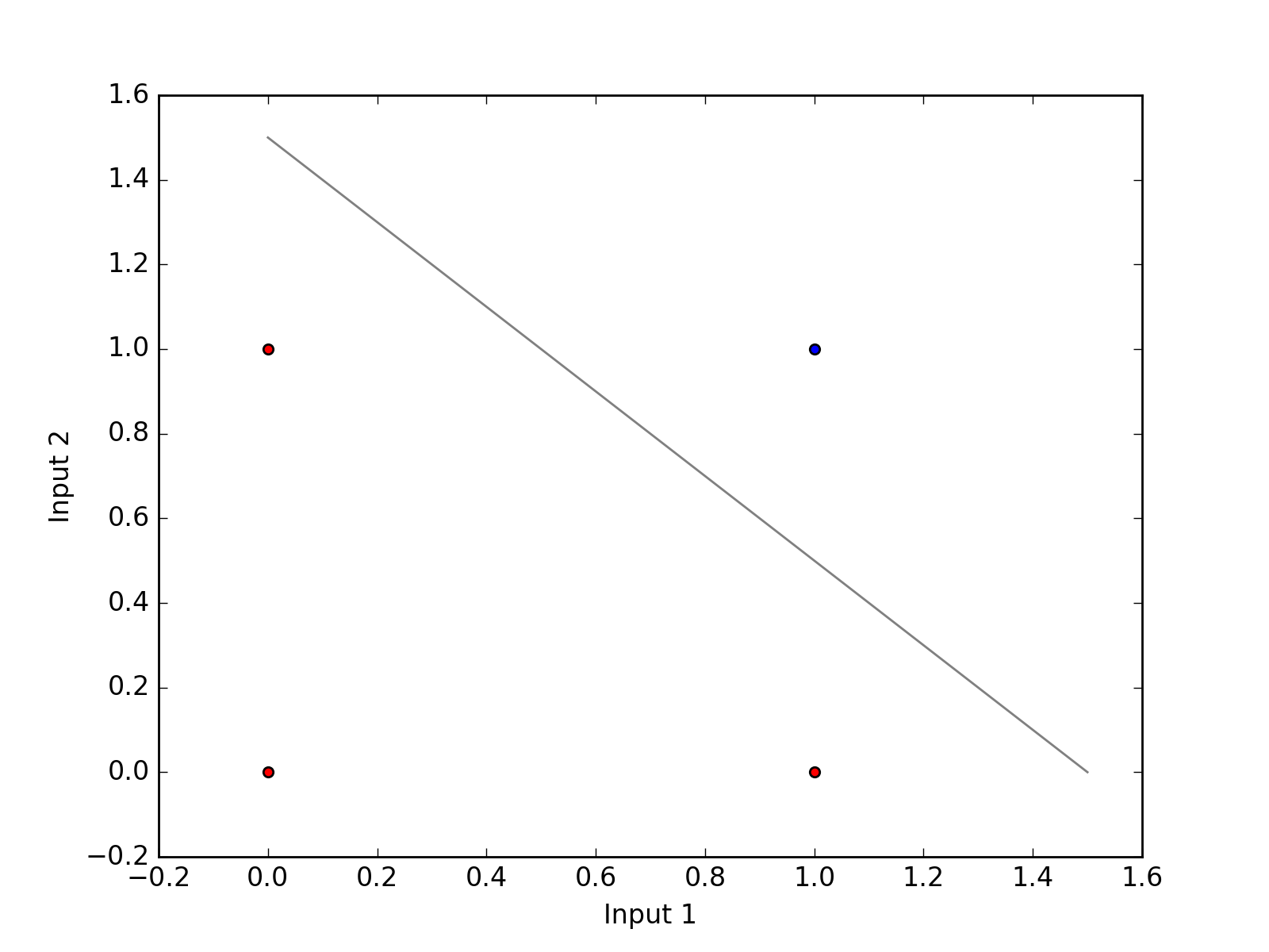
Input 1 Input 2 Output

0 0 0

0 1 0

1 0 0

1 1 1

In order to answer the question, whether out hypothesis set is big enough to model the AND-gate, it is helpful to represent the above table as a graph similar to the iris data above.

The features of each data point \(x^{(i)}\) are the two input signals and the output value 0 and 1 are encoded by the class labels \(y^{i}\in\{-1,+1\}\).

(Source code, png, hires.png, pdf)

The colors: red and blue denote the output values 0 or 1 of the AND-gate.;

Note that the data points a linearly seperable;

Note that these two classes of data points can be well separated by a hyperplane (in this case a line ☺). Hence, it is easy to find a good weight vector \(w\). For instance:

(2)¶\[\begin{split}w = \begin{pmatrix} -1.5\\ 1\\ 1 \end{pmatrix}.\end{split}\]

Homework

Check if \(f\) in (1) with the weight vector given in (2) decribes an AND-gate correctly and note that \(w\) is by no means unique.

Give a geometric interpretation of the \(w\).

Check all 16 bitwise logic gates and note which can be ‘learned’ by the model (1) and which not – in the latter case, discuss why not.

3.2.1. Learning rule¶

Having settled for a hypothesis set such as \(f\) in (1), the task is to learn a good parameters, i.e., in our case a good weight vector \(w\), in the sense discussed in the previous section.

This is now done by adjusting the weight vector \(w\) appropriately depending on the training data \((x^{(i)},y^{(i)})_{1\leq i\leq M\leq N}\),
in a way that minimizes the classification errors, i.e., the number of indices \(i\) for which \(f(x^{(i)})\neq y^{(i)}\).

The algorithm by which the ‘learning’ is facilitated shall be called learning rule and can be spell out as follows:

INPUT: Pre-labeled training data \((x^{(i)},y^{(i)})_{1\leq i\leq M\leq N}\)

STEP 1: Initialize the weight vector \(w\) to zero or conveniently distributed random coefficients.

STEP 2: Pick a data point \((x^{(i)},y^{(i)})\) in the training samples at random:

Compute the output

\(y = f(x^{(i)})\)

Compare \(y\) with \(y^{(i)}\):

If \(y=y^{(i)}\), go back to STEP 2.

Else, update the weight vector \(w\) appropriately according to an update rule, and go back to STEP 2.

The following sketch is a visualization of the feedback loop for the learning rule:

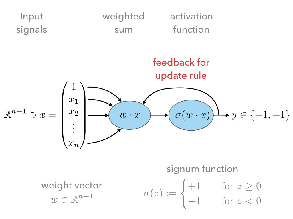
The important step is the update rule which we discuss next.

3.2.2. Update rule¶

Let us spell out a possible update rule and then discuss why it does what we want:

First, we compute the difference between the correct label \(y^{(i)}\) given by the training data and the prediction \(y=f(x^{(i)})\):

(3)¶\[\Delta^{(i)} := y^{(i)} - y\]

Second, we perform an update of the weight vector as follows:

(4)¶\[w \mapsto \tilde w := w + \delta w\]

where

(5)¶\[\delta w := \eta \, \Delta^{(i)} \, x^{(i)}.\]

The parameter \(\eta\in\mathbb R^+\) is called ‘learning rate’.

Why does this update rule lead to a good choice of weights \(w\)?

Assume that in STEP 2 b. of the learning rule identified a misclassification and calls the update rule. There are two possibilities:

\(\Delta=2\): This means that the model predicted \(y=-1\) although the correct label is \(y^{(i)}=1\).

Hence, by definition of \(f\) in (1) the value of \(w\cdot x^{(i)}\) is too low;

This can be fixed by adjusting the weights according to (4) and (5);

Next time when this data point is examined one finds

\[\begin{split}\tilde w \cdot x^{(i)} &= (w + \delta w)\cdot x^{(i)}\\ &= w \cdot x^{(i)} + \eta \, \Delta \, (x^{(i)})^2 &\geq w \cdot x^{(i)}\end{split}\]

because, as \(\Delta > 0\) and the square is non-negative, the last summand on the right is positive.

Hence, the new weight vector is changed in such a way that, next time, it is more likely that \(f\) will predict the label of \(x^{(i)}\) correctly.

\(\Delta=-2\): This means that the model predicted \(y=1\) although the correct label is \(y^{(i)}=-1\).

By the same reasoning as in case 1. one finds:

\[\begin{split}\tilde w \cdot x^{(i)} &= (w + \delta w)\cdot x^{(i)}\\ &= w \cdot x^{(i)} + \eta \, \Delta \, (x^{(i)})^2 &\leq w \cdot x^{(i)}\end{split}\]

because now we have \(\Delta < 0\), and again, the correction works in the right direction.

The model (1) for \(f\), i.e., hypothesis set, and this particular learning and update rule is what defines the ‘Perceptron’.

3.2.3. Convergence¶

Now that we have a heuristic understanding why the learning and update rule chosen for the Perceptron works, we have a look at what can be said mathematically; see [varga_neural_1996] for a more detailed discussion.

First let us make precise what we mean by ‘linear separability’:

Definition: (Linear seperability) Let \(A,B\) be two sets in \(\mathbb R^n\). Then:

\(A,B\) are called linearly seperable iff there is a

\(w\in\mathbb R^{n+1}\) such that

\[\forall\, \mathbf a\in A,\,\mathbf b\in B: \quad w\cdot a \geq 0 \quad \wedge \quad w\cdot b < 0.\]
\(A,B\) are called absolutely linearly seperable iff there is a

\(w\in\mathbb R^{n+1}\) such that

\[\forall\, \mathbf a\in A,\,\mathbf b\in B: \quad w\cdot a > 0 \quad \wedge \quad w\cdot b < 0.\]

The learning and update rule algorithm of the Perceptron can be formulated in terms of the following algorithm:

Algorithm: (Perceptron)

PREP:

Prepare the training data \((\mathbf x^{(i)},y^{(i)})_{1\leq i\leq M}\). Let \(A\) and \(B\) be the sets of elements \(x^{(i)}\in\mathbb R^{n+1}=(1,\mathbb x^{(i)})\) whose class labels fulfill \(y^{(i)}=+1\) and \(y^{(i)}=-1\), respectively.

START:

Initialize the weight vector \(w^{(0)}\in\mathbb R^{n+1}\) with random numbers and set \(t:=0\).

STEP:

Choose \(x\mathbb \in A,B\) at random:

If \(x\in A, w^{(t)}\cdot x \geq 0\): goto STEP.

If \(x\in A, w^{(t)}\cdot x < 0\): goto UPDATE.

If \(x\in B, w^{(t)}\cdot x \leq 0\): goto STEP.

If \(x\in B, w^{(t)}\cdot x > 0\): goto UPDATE.

UPDATE:

If \(x\in A\), then set \(w^{(t+1)}:=w^{(t)} + x\), increment \(t\mapsto t+1\), and goto STEP.

If \(x\in B\), then set \(w^{(t+1)}:=w^{(t)} - x\), increment \(t\mapsto t+1\), and goto STEP.

Note that for an implementation of this algorithm we will also need an exit criterion so that the algorithm does not run forever.
This is usually done by specifying how many times the entire training set is run through STEP, a number which is often referred to as number of epochs.
Note further, that for sake of brevity , the learning rate \(\eta\) was chosen to equal \(1/2\).

Frank Rosenblatt already showed convergence of the algorithm above in the case of finite and linearly separable training data:

Theorem: (Perceptron convergence)

Let \(A,B\) be finite sets and linearly seperable, then the number of updates performed by the Perceptron algorithm stated above is finite.

As a first step, we observe that since \(A,B\) are finite sets that are linear seperable, they are also absolutely seperable due to:

Proposition:

Let \(A,B\) be finite sets of \(\mathbb R^{n+1}\): \(A,B\) are linearly seperable \(\Leftrightarrow\) \(A,B\) are absolutely linearly seperable.

Homework.

Furthermore, we observe that without restriction of generality (WLOG) we may assume the vectors \(x\in A\cup B\) to be normalized because

\[w\cdot x > 0 \, \vee \, w\cdot x < 0 \Leftrightarrow w\cdot \frac{x}{\|x\|} > 0 \, \vee \, w\cdot \frac{x}{\|x\|} < 0.\]
Let us define \(T=A\cup (-1)B\), i.e., \(T\) is the union of \(A\) and the element of \(B\) times \((-1)\).
Since \(A,B\) absolutely linearly seperable there is a \(w^*\in\mathbb R^{n+1}\) such that for all \(x\in T\)

(6)¶\[w^{*}\cdot x > 0.\]

And moreover, we also may WLOG assume that \(w^{*}\) is normalized.

Let us assume that some time after the \(t\)-th update a point \(x\in T\) is picked in STEP that leads to a misclassification

\[w^{(t)} \cdot x < 0\]

so that UPDATE will be called which updates the weight vector according to

\[w^{(t+1)} := w^{(t)} + x.\]

Note that both cases of UPDATE are treated with this update since in the definition of \(T\) we have already included the ‘minus’ sign.

Now in order to infer a bound on the number of updates \(t\) in the Perceptron algorithm above, consider the quantity

(7)¶\[1\leq \cos \varphi = \frac{w^{*}\cdot w^{(t+1)}}{\|w^{(t+1)}\|}.\]

To bound this quantity also from below, we consider first:

\[w^{*}\cdot w^{(t+1)} = w^{*}\cdot w^{(t)} + w^{*}\cdot x.\]

Thanks to (6) and the finiteness of \(A,B\), we know that

\[\delta := \min\{w\cdot x \,|\, x \in T\} > 0.\]

This facilitates the estimate

\[w^{*}\cdot w^{(t+1)} \geq w^{*}\cdot w^{(t)} + \delta,\]

which, by induction, gives

(8)¶\[w^{*}\cdot w^{(t+1)} \geq w^{*}\cdot w^{(0)} + (t+1)\delta.\]

Second, we consider the denumerator of (7):

\[\| w^{(t+1)} \|^2 = \|w^{(t)}\|^2 + 2 w^{(t)}\cdot x + \|x\|^2.\]

Recall that \(x\) was misclassified by weight vector \(w^{(t)}\) so that \(w^{(t)}\cdot x<0\). This yields the estimate

\[\| w^{(t+1)} \|^2 \leq \|w^{(t)}\|^2 + \|x\|^2.\]

Again by induction, and recalling the assuption that \(x\) was normalized, we get:

(9)¶\[\| w^{(t+1)} \|^2 \leq \|w^{(0)}\|^2 + (t+1).\]

Both bounds, (8) and (9), together with (7), give rise to the inequalities

(10)¶\[1 \geq \frac{w^{*}\cdot w^{(t+1)}}{\|w^{(t+1)}\|} \geq\frac{w^{*}\cdot w^{(0)} + (t+1)\delta}{\sqrt{\|w^{(0}\|^2 + (t+1)}}.\]

The right-hand side would grow \(O(\sqrt t)\) but has to be smaller one. Hence, \(t\), i.e., the number of updates, must be bounded by a finite number.

What is the geometrical meaning of \(\delta\) in (3) in the proof above?
Consider the case \(w^{(0)}=0\) and give an upper bound on the maximum number of updates.
Carry out the analysis above including an arbitrary learning rate \(\eta\). How does \(\eta\) influence the number of updates?

Finally, though this result is reassuring it needs to be emphasized that it is rather academic.

The convergence theorem only holds in the case of linear separability of the test data, which in most interesting cases is not given.

3.2.4. Python implementation¶

Next, we discuss an Python implementation of the Perceptron discussed above.

The mathematical model of the function \(f\), i.e., the hypothesis set, the learning and update rule will be implemented as a Python class:

class Perceptron:

    def __init__(self, num):
        '''
        initialize class for `num` input signals
        '''

        # weights of the perceptron, initialized to zero
        # note the '1 + ' as the first weight entry is the threshold
        self.w_ = np.zeros(1 + num)

        return

The constructor __init__ takes as argument the number of input signals num and initializes the variable w_ which will be used to store the weight vector \(w\in\mathbb R^{n+1}\) where \(n=\) num.

The constructor is called when an object of the Perceptron class is created, e.g., by:
```
ppn = Perceptron(2)
```
In this example, it initializes a Perceptron with \(n=2\).
The first method activation_input of the Perceptron class takes as argument an array of data points X, i.e., \((x^{(i)})_i\), and returns the array of input activations \(w\cdot x^{(i)}\) for all \(i\) using the weight vector \(w\) stored in variable w_:
1 2 3 4 5
def activation_input(self, X): ''' calculate the activation input of the neuron ''' return np.dot(X, self.w_[1:]) + self.w_[0]
The second method classify takes again an array of data points X, i.e., \((x^{(i)})_i\) as argument. It uses the previous method input_activation to compute the input activations \((w\cdot x^{(i)})_i\) and then applies the signum function to the values in the arrays:
1 2 3 4 5
def classify(self, X): ''' classify the data by sending the activation input through a step function ''' return np.where(self.activation_input(X) >= 0.0, 1, -1)
This method is the implantation of the function \(f\) in (1).

Finally, the next method implements the learning and update rule:

def learn(self, X_train, Y_train, eta=0.01, epochs=10):
    '''
    fit training features X_train with labels Y_train according to learning rate
    `eta` and total number of epochs `epochs` and log the misclassifications in errors_
    '''

    # reset internal list of misclassifications for the logging
    self.train_errors_ = []

    # repeat `epochs` many times
    for _ in range(epochs):
        err = 0
        # for each pair of features and corresponding label
        for x, y in zip(X_train, Y_train):
            # compute the update for the weight coefficients
            update = eta * ( y - self.classify(x) )
            # update the weights
            self.w_[1:] += update * x
            # update the threshold
            self.w_[0] += update
            # increment the number of misclassifications if update is not zero
            err += int(update != 0.0)
        # append the number of misclassifications to the internal list
        self.train_errors_.append(err)

    return

It takes as input arguments the training data \((x^{(i)},y^{(i)})_{1\leq i\leq M}\) in form of two arrays X_train and Y_train, and furthermore, the learning rate eta, i.e., \(\eta\), and an additional number called epochs.
The latter number epochs specifies how many times the learning rule runs over the whole training data set – see the for loop in line number 11.
In the body of the first for loop a variable err is set to zero and a second for loop over set of training data points is carried out.
The body of the latter for loop implement the update rule (3)-(5).
Note that there are two types of updates, i.e., lines 18 and 20. This is due to the fact that above we used the convention that the first coefficient of \(x\) was fixed to one in order to keep the notation slim.
In line 22 err is incremented each time a misclassification occurred. The number of misclassification per epoch is then append to the list train_errors.

After loading to training data set \((x^{(i)},y^{(i)})_{1\leq i\leq M}\) into the two arrays X_train and Y_train the Perceptron can be initializes and trained as follows:

ppn = Perceptron(X.shape[1])
ppn.learn(X_train, Y_train, eta=0.1, epochs=100)

Find the full implementation here: [Link]

Have a look at the Perceptron implementation (link given above):

a. What effect does the learning rate have? Examine a situation is which the learning rate is too high and too low and discuss both cases.

b. What happens when the training data cannot be separated by a hyperplane? Examine problematic situation and discuss these – for example, by generating fictitious data points.

c. Note that the instant all training data was classified correctly the Perceptron stops to update the weight vector. Is this a feature or a bug?

d. Discuss the dependency of the learning success on the order in which the training data is presented to the Perceptron. How could the dependency be suppressed?

3.2.5. Problems with the Perceptron¶

As discussed, the convergence of the Perceptron algorithm is only guaranteed in the case of linearly separable test data.
If linear separability is not provided, in each epoch will be at least one update.
Thus, in general we need a good exit criterion for the algorithm to bound the maximum number of updates.
The updates stop the very instant the entire test data is classified correctly, which might lead to poor generalization properties of the resulting classifier to unknown data.

3.3. Adaline¶

The Adaline algorithm will overcome some of the short-comings of the one of Perceptron.
The basic design is almost the same:
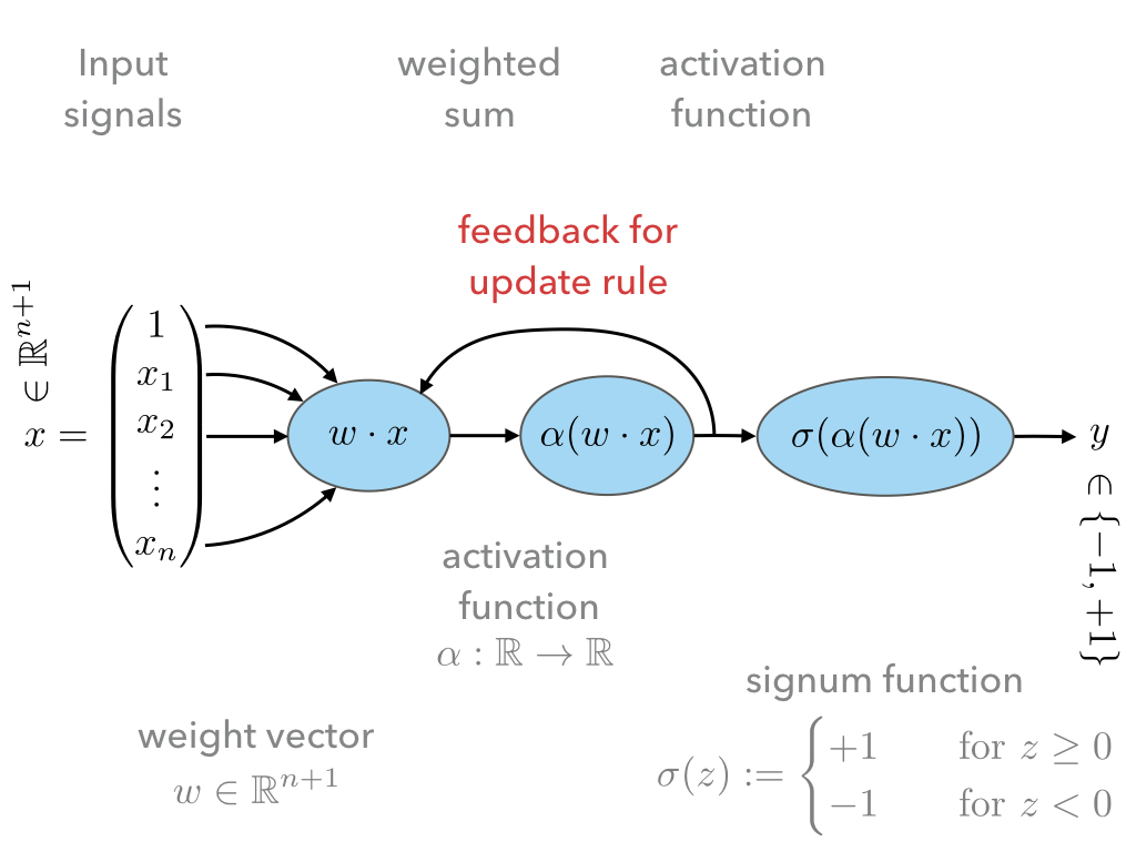
The first difference w.r.t. to the Perceptron is the additional activation function \(\alpha\). We shall call \(w\cdot x\) activation input and \(\alpha(w\cdot x)\) activation output.
We will discuss different choices of activation functions later. For now let us simply use:

\[\alpha(z)=z.\]
The second difference is that the activation output is used as in feedback loop for the update rule.
The advantage is that, provided \(\alpha:\mathbb R\to\mathbb R\) is regular enough, we may make use of analytic optimization theory in order to find an in some sense ‘optimal’ choice of weights \(w\in\mathbb R^{n+1}\).
This was not possible in the case of the Perceptron because the signum function is not differentiable.

3.3.1. Update rule¶

Recall that an ‘optimal’ choice of weights \(w\in\mathbb R^{n+1}\) should fulfill two properties:
1. It should ‘accurately’ classify the training data \((x^{(i)},y^{(i)})_{1\leq i\leq M}\),
2. and it should ‘generalize’ well unknown data.
In order to make use of analytic optimization theory, one may attempt to encode the quality of weights w.r.t. these two properties in form of a function that attains smaller and smaller values the better the weights fulfill these properties.
This function is called many names, e.g., ‘loss’, ‘regret’, ‘cost’, ‘energy’, or ‘error’ function. We will use the term ‘loss function’.
Of course, depending on the classification task, there are many choice. Maybe one of the simplest examples:

(11)¶\[L(w) := \frac12 \sum_{i=1}^M \left(y^{(i)} - \alpha(w\cdot x^{(i)})\right)^2,\]

which is the accumulated squarred euclidean distance between the particular labels of the test data \(y^{(i)}\) and the corresponding prediction \(\alpha(w\cdot x^{(i)})\) given by Adaline for the current weight vector \(w\).
Note that the loss function depends not only on \(w\), but also on the entire training data set \((x^{(i)},y^{(i)})_{1\leq i\leq M}\). The latter, however, is assumed to be fixed which is why the dependence of \(L(w)\) on it will be suppressed in out notation.
From its definition the loss function in (11) has the desired property that it grows and decreases whenever the number of misclassification grows or decreases, respectively.
Furthermore, it does so smoothly, which allows for the use of analytic optimization theory.

3.3.2. Learning and update rule¶

Having encoded the desired properties of ‘optimal’ weights \(w\in\mathbb R^{n+1}\) as a global minimum of the function \(L(w)\), the only task left to do is to find this global minimum.
Depending on the function \(L(w)\), i.e., on the training data, this task may be arbitrarily simple or difficult.
Consider the following heuristics in order to infer a possible learning strategy:
- Say, we start with a weight vector \(w\in\mathbb R^{n+1}\) and want to make an update
  
  \[w\mapsto \tilde w:=w + \delta w\]
  
  in a favourable direction \(\delta w\in\mathbb R^{n+1}\).
- An informal Taylor expansion of \(L(\tilde w)\) reveals
  
  \[L(\tilde w) = L(w) + \frac{\partial L(w)}{\partial w} \delta w + O(\delta w^2).\]
- In order to make the update ‘favourable’ we want that \(L(\tilde w)\leq L(w)\).
- Neglecting the higher orders, this would mean:
  
  (12)¶\[\frac{\partial L(w)}{\partial w} \delta w < 0.\]
- In order to get rid of the unknown sign of \(\frac{\partial L(w)}{\partial w}\) we may choose:
  
  (13)¶\[\delta w := - \eta \frac{\partial L(w)}{\partial w}\]
  
  for some learning rate \(\eta\in\mathbb R^+\).
- Note that for the choice (13) the linear order (12) becomes negative and therefore works to decrease the value of \(L(w)\).

Concretely, for our case we find:

\[\frac{\partial L(w)}{\partial w} = -\sum_{i=1}^M \left( y^{(i)}-\alpha(w\cdot x^{(i)}) \right) \alpha'(w\cdot x^{(i)}) x^{(i)}.\]

Hence, we may formulate the Adaline algorithm as follows:

INPUT: Pre-labeled training data \((x^{(i)},y^{(i)})_{1\leq i\leq M\leq N}\)

STEP 1: Initialize the weight vector \(w\) to zero or conveniently distributed random coefficients.

STEP 2: For a certain number of epochs:

Compute \(L(w)\)

Update the weights \(w\) according to

\[w \mapsto \tilde w := w + \eta \sum_{i=1}^M \left( y^{(i)}-\alpha(w\cdot x^{(i)}) \right) \alpha'(w\cdot x^{(i)}) x^{(i)}\]

Prove that even in the linearly seperable case, the above Adaline algorithm does not need to converge. Do this by constructing a simple example of training data and a special choice of learning rate \(\eta\).
What is the influence of large or small values of \(\eta\)?
Discuss the advantages/disadvantages of immediate weight updates after misclassification as it was the case for the Perceptron and batch updates as it is the case for Adaline.

3.3.3. Python implementation¶

As we have already noted, the Adaline learning rule is the same as the one of the Perceptron. Hence, we only need to change the learning rule implemented in the method learn of the Perceptron class. The Adaline class can therefore we created as follows:

class Adaline(Perceptron):

    def learn(self, X_train, Y_train, eta=0.01, epochs=1000):
        '''
        fit training data according to eta and n_iter
        and log the errors in errors_
        '''

        # we initialize two list, each for the misclassifications and the cost function
        self.train_errors_ = []
        self.train_loss_ = []

        # for all the epoch
        for _ in range(epochs):
            # classify the traning features
            Z = self.classify(X_train)
            # count the misqualifications for the logging
            err = 0
            for z, y in zip(Z, Y_train):
                err += int(z != y)
            # ans save them in the list for later use
            self.train_errors_.append(err)

            # compute the activation input of the entire traning features
            output = self.activation_input(X_train)
            # and then the deviation from the labels
            delta = Y_train - output
            # the following is an implmentation of the adaline update rule
            self.w_[1:] += eta * X_train.T.dot(delta)
            self.w_[0] += eta * delta.sum()
            # and finally, we record the loss function
            loss = (delta ** 2).sum() / 2.0
            # and save it for later use
            self.train_loss_.append(loss)

        return

Line 1 defines the Adaline class and a child of the Perceptron one. It thus inherits all the methods and variables of the Perceptron class.
Line 11 introduces a similar variable as train_errors that will store the value of the loss function per epoch.
Line 14 is again the for loop over the epochs:
In line 16 the classification of all training data points is conducted.
Lines 17-22 only count the number of misclassification which is then appended to the list train_errors_.
The update rule is implemented in Lines 24-30. First, the input activation of all the training data is computed and the array delta stores the set \((y^{(i)}-w \cdot x^{i)})\).
This delta array is then used to compute the updated weight vector stored in w_ in lines 29-30.
The last two lines in this for loop compute the loss value for this epoch and store it in the list train_loss_.

Find the full implementation here: [Link]

3.3.4. The learning rate parameter and preparation of training data¶

We have introduced the learning rate \(\eta\) in an ad-hoc fashion;
Not even in the linear separable case, we may expect convergence of the Adaline algorithm;
We can only expect to find a good approximation of the optimal choice of weights \(w\in\mathbb R^{n+1}\);
But this will depend on the choice of the learning rate parameter.

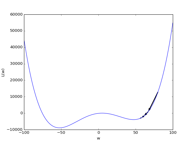
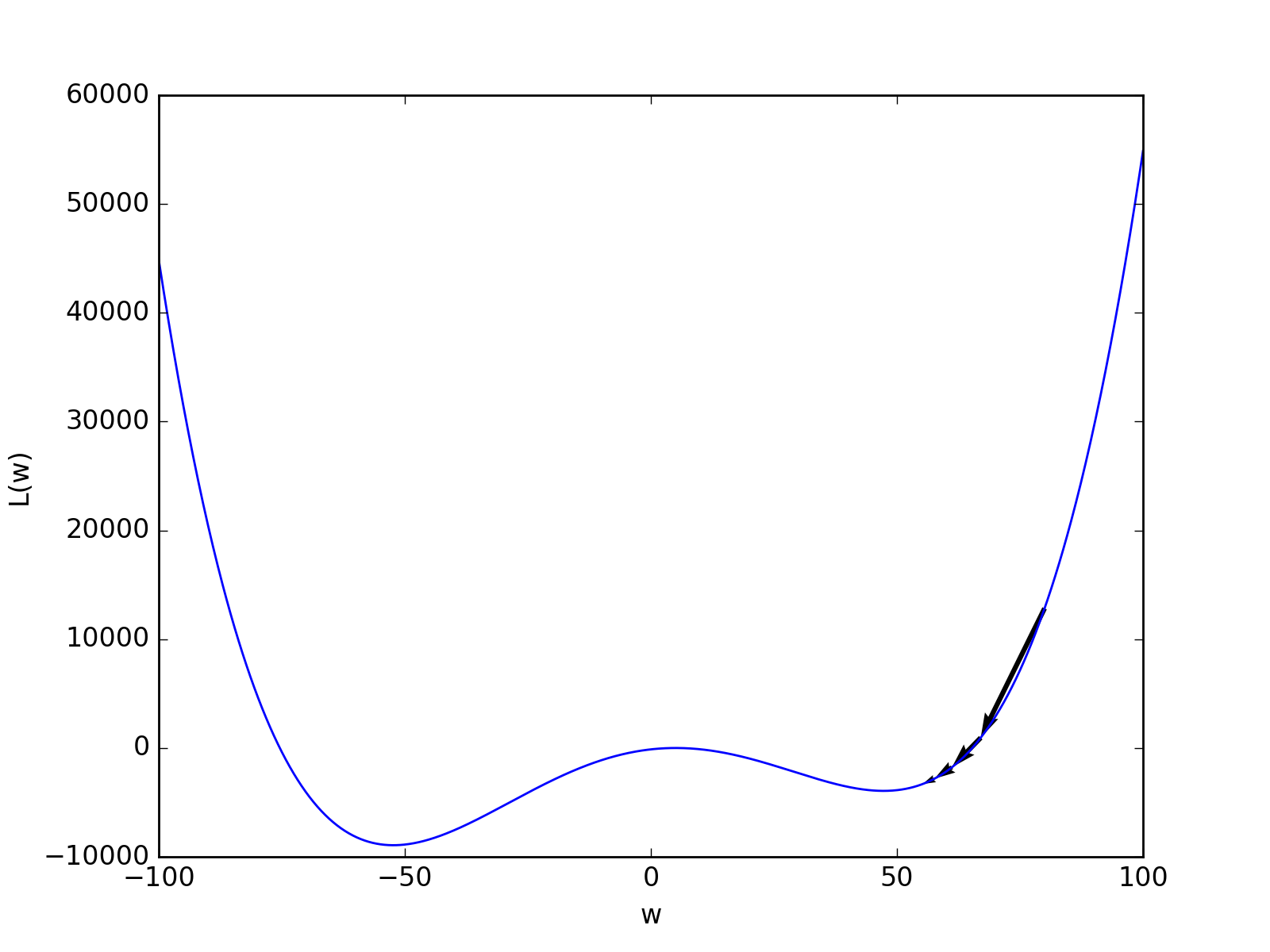
In the figure below, the learning rate \(\eta\) was chosen too large. Instead of approximating the minimum value, the gradient descent algorithm even diverges.

(Source code, png, hires.png, pdf)

In the next figure, the learning rate \(\eta\) has been chosen too small. In case, the loss function has other local minima, the initial weight vector \(w\) is coincidently chosen near such a local minimum, and the learning rate is too small, the gradient descent algorithm will converge too the nearest local minimum instead of the global minimum.

(Source code, png, hires.png, pdf)

In the special case of a linear activation \(\alpha(z)=z\) and a quadratic loss function such as (11), which we also used in our Python implementation, such a behavior cannot occur due to convexity. In more general settings that we will discuss later, a multitude of local minima can, however, be the generic case.

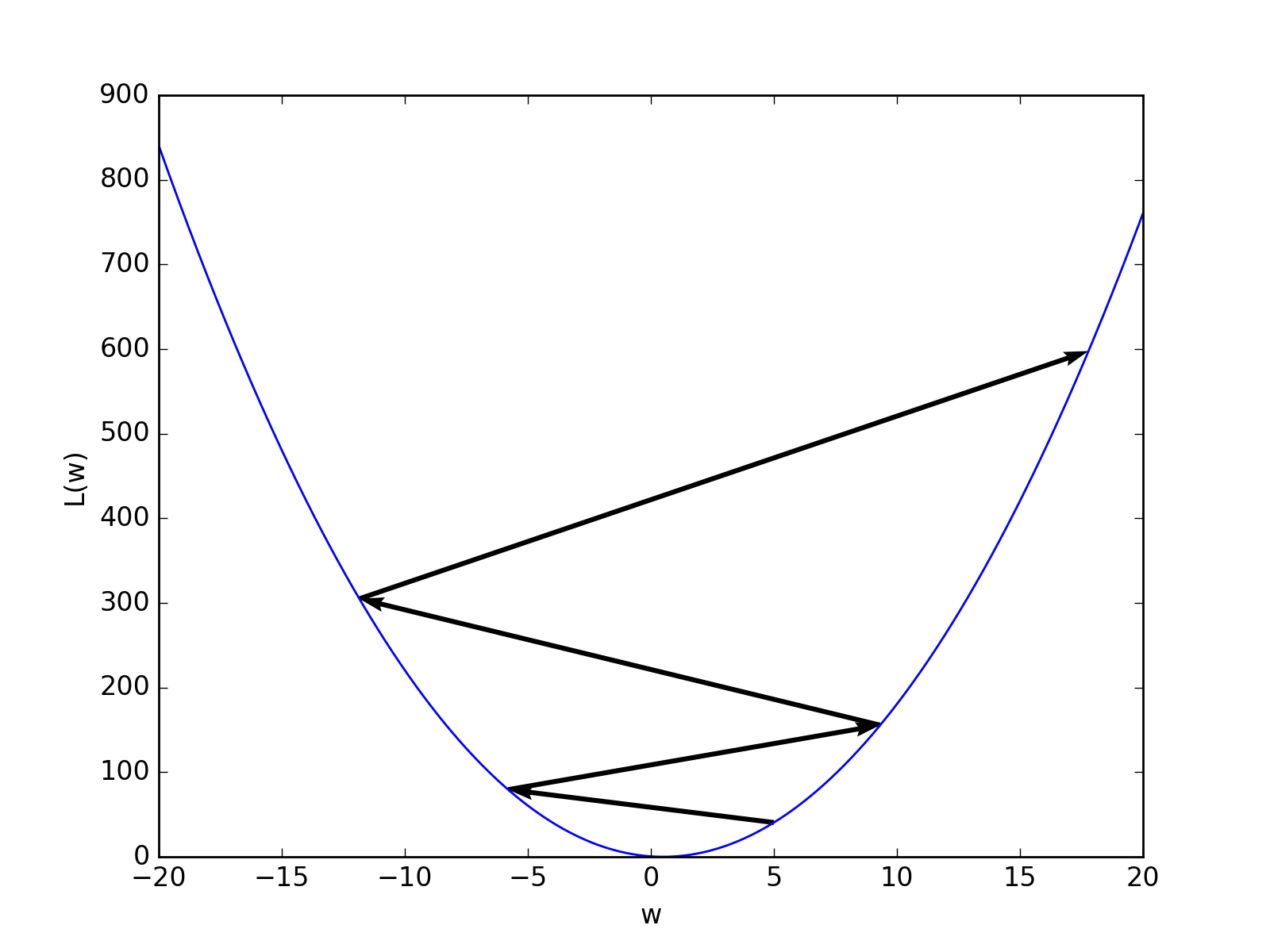
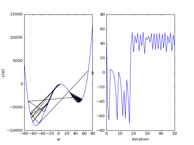
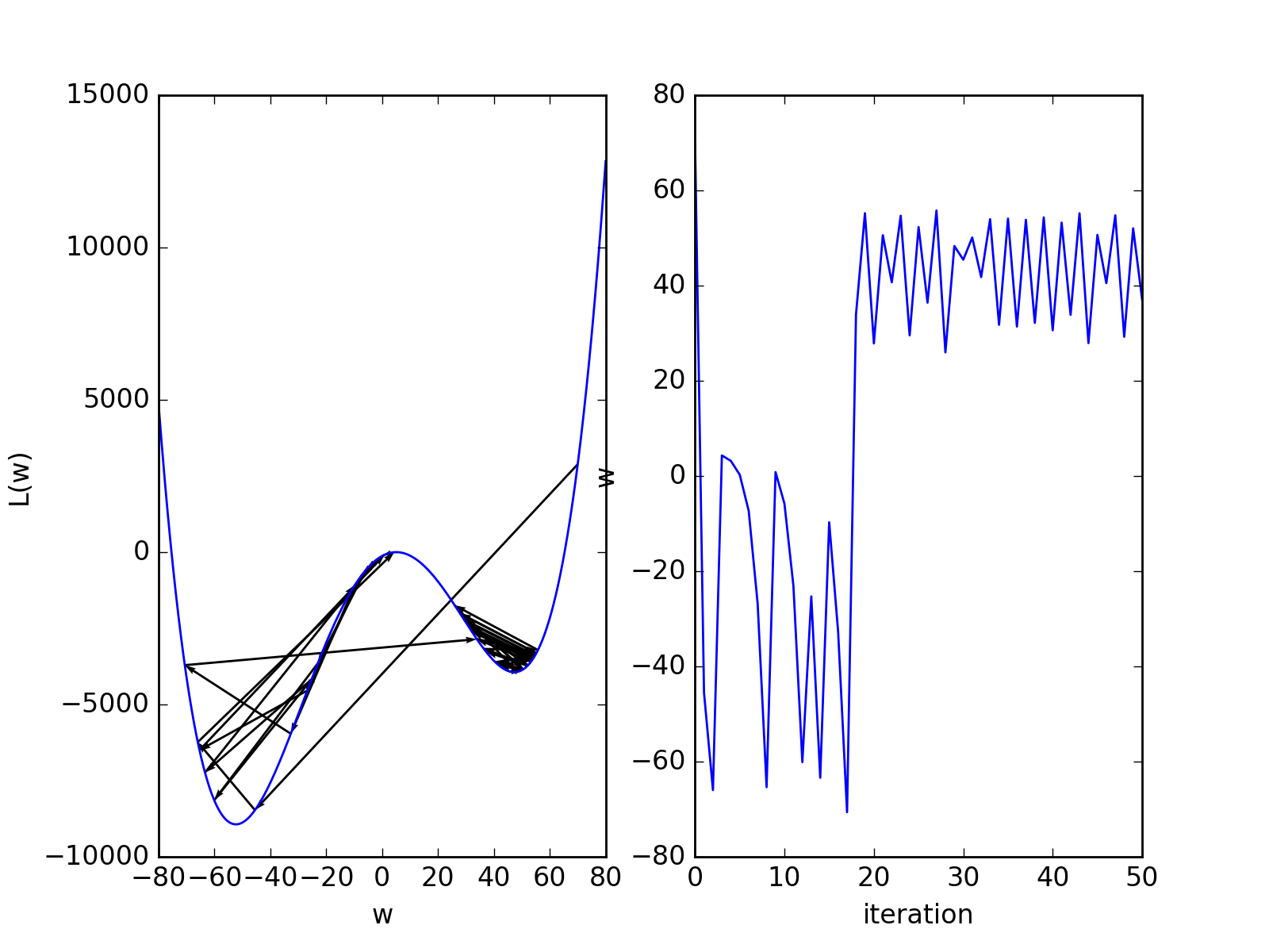
Here is another bad scenario where we see that the gradient descent algorithm does not converge:

(Source code, png, hires.png, pdf)

_images/learning_rate_no_convergence.png

Many improvements can be made with respect to the gradient descent algorithms which tend to work well in different situations. Here is a nice overview on popular optimization algorithms used in machine learning: [URL]

In general, the learning rate \(\eta\) will depend very much on the fluctuations in the features of your training data set. In order, to have comparable results it is therefore a good idea to normalize the training data. A standard procedure to do this is to transform the training data according to the following map

\[x^{(i)} \mapsto \widetilde x^{(i)} := \frac{x^{(i)} - \mu}{\sigma},\]

where

\[\mu:=\frac1M\sum_{i=1}^M x^{(i)}\]

is the empirical average and

\[\sigma:=\sqrt{\frac1M\sum_{i=1}^M (x^{(i)} - \mu)}\]

is the standard variation.

3.3.4.1. Online learning versus batch learning¶

The learning and update rule of the Perceptron and Adaline have a crucial difference:
- The Perceptron updates its weights according to inspection of a single data point \((x^{(i)},y^{(i)})\) of the training data \((x^{(i)},y^{(i)})_{1\leq i\leq M}\) – this is usually referred to as ‘online’ (in the sense of ‘real-time’) or ‘stochastic’ (in the sense that training data points are chosen at random) learning.
- The Adaline conducts an update after inspecting the whole training data \((x^{(i)},y^{(i)})_{1\leq i\leq M}\) by means of computing the gradient of the loss function (11) that depends on the entire set of training data – this is usually referred to as ‘batch’ learning (in the sense that the whole batch of training data is used to compute an update of the weights).
While online learning has a strong dependence on the sequence of training data points presented to the learner, batch learning can become computationally very expensive.
A compromise between them two extremes is the so-called ‘mini-batch’ learning.
- The entire batch of training data \(I=(x^{(i)},y^{(i)})_{1\leq i\leq M}\) is then split up into disjoint mini-batches \(I_k:=(x^{(i)},y^{(i)})_{i_{k-1}\leq i\leq i_{k}}\) for an appropriate strictly increasing sequence of indices \((i_k)_k\) such that \(I=\bigcup_k I_k\).
- For each mini-batch \(I_k\) the mini-batch loss function is computed
  
  \[L(w) := \frac12 \sum_{i=i_{k-1}}^{i_k-1} \left(y^{(i)} - \alpha(w\cdot x^{(i)})\right)^2,\]
  
  and the update of the weight vector \(w\) is performed acordingly.
For appropriate chosen mini-batch sizes this mini-batch learning rule often proves to faster than online or batch learning.

Turn our Adaline implementation into a mini-batch learner.

3.3.4.2. Where to go from here?¶

The step from the Perceptron to Adaline mainly brings two advantages:

We may make use of analytic optimization theory;
We may encode what we mean by ‘optimal’ weights \(w\), i.e., by the terms ‘accurately’ and ‘generalizes’ of the introductory discussion, by the choice of the corresponding loss function.

This freedom leads to a rich class of linear classifiers, parametrized by the choice of activation function \(\alpha(z)\) and the form of loss function \(L(w)\).

Discuss how the ‘optimal’ choice of weights is influence by changing the loss function (11) to

\[L(w) := \|w\|_p + \frac12 \sum_{i=1}^M \left(y^{(i)} - \alpha(w\cdot x^{(i)})\right)^2,\]

where \(\|w\|_p := (\sum_i |w_i|^p)^{1/p}\) is the usual \(L^p\)-norm for \(p\in \mathbb N\cup\{\infty\}\).
What properties should the loss function quite generally fulfill in order to employ analytic optimization theory?

In the next chapter we shall look at one of the most important example of such models, the so-called ‘support vector machine’ (SVM).

3.4. Support Vector Machine¶

While the Adaline loss function was good a measure of how accurately the training data is classified, it did not put a particular emphasis on how the optimal weights \(w\) may generalize for the training data to unseen data;
Next, we shall specify such a sense and derive a corresponding loss function;

3.4.1. Linear seperable case¶

Consider a typical linear seperable case of training data. Depending on the initial weights both, the Adaline and Perceptron, may find different separation hyperplanes of the same training data, however, among all of the possible seperation hyperplanes there is a special one:
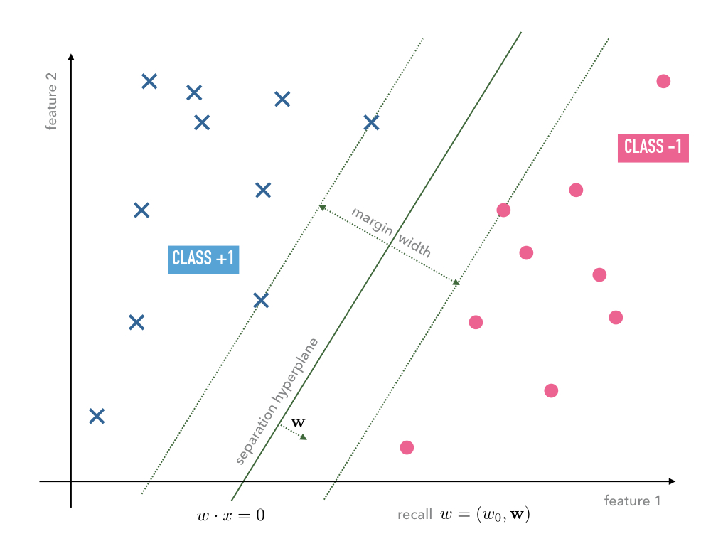
The special seperation hyperplane maximizes the margin width of the seperation.
Note that the minimal distance of a point \(x\) and the separation hyperplane defined by \(w\) is given by

\[\operatorname{dist_w}(x) := \frac{|w\cdot x|}{\|\mathbf w\|};\]

recall that \(w=(w_0,\mathbf w)\).
Furthermore, note that the separation of the training data into the classes +1 and -1 given by the signum of \(w\cdot x^{(i)}\) is scale invariant.

Todo

Under construction. See for example [vapnik_statistical_1998], [mohri_foundations_2012].

Distance between point and hyperplane in normal form.
Scale invariance of \(w\cdot x=0\).
Minimization problem has a unique solution.

3.4.2. Soft margin case¶

Todo

Under construction. See for example [vapnik_statistical_1998], [mohri_foundations_2012].

Minimization problem still has a unique solution.
Meaning of slack variables.