Where to go from here?¶

The step from the Perceptron to Adaline mainly brings two advantages:

We may make use of analytic optimization theory;
We may encode what we mean by ‘optimal’ weights $w$ , i.e., by the terms ‘accurately’ and ‘generalizes’ of the introductory discussion, by the choice of the corresponding loss function.

This freedom leads to a rich class of linear classifiers, parametrized by the choice of activation function $\alpha(z)$ and the form of loss function $L(w)$ . As there is great freedom in this choice we must understood better how we can encode certain learning objectives in this choice. We shall look in more detail at two different choice from (11) and (12) in the next chapters. One of them results in the industry-proven ‘support vector machine’ (SVM) model.

Discuss how the ‘optimal’ choice of weights is influence by changing the loss function (12) to

$L(w) := \|w\|_p + \frac12 \sum_{i=1}^M \left(y^{(i)} -\alpha(w\cdot x^{(i)})\right)^2,$

where $\|w\|_p := (\sum_i |w_i|^p)^{1/p}$ is the usual $L^p$ -norm for $p\in \mathbb N\cup\{\infty\}$ .
Give an example of a loss function employing a notion of distance other than the Euclidean one and implement the corresponding Adaline.

Sigmoid activation function¶

One of the widely employed choices in machine learning models that are based on the Adaline framework are sigmoid functions. This class of functions is usually defined as bouded differentiable function $\mathbb R\to\mathbb R$ with a non-negative derivative. Two frequent examples are the logistic function

(18)¶ $\alpha: \mathbb Z \to [0,1], \qquad \alpha(z):=\frac{1}{1+e^{-z}}$

and the hyperbolic tangent

$\alpha: \mathbb Z \to [-1,1], \qquad \alpha(z):=\tanh(z) = \frac{e^z-e^{-z}}{e^z+e^{-z}}.$

Prove that any sigmoid function has a pair of two horizontal asymptodes for $x\to\pm\infty$ .

Compared to the linear activation in (11) these functions often have several advantages.

First, their ranges are bounded by definition. In the cases considered above, in which there are only two class labels, say or $\{0,1\}$ or $\{-1,+1\}$ , the linear activation function (11) may attain values much lower or higher that the numbers used to encode the class labels. This may lead to extreme updates according to the update rule (16) as the difference $(y^{(i)}-\alpha(w\cdot x^{(i)}))$ may become very large. In the Adaline case considered above in which we only had one output signal we did not encounter problems during training because of such potentially large signals. On the contrary they were rather welcome as they pushed the weight vector strongly in the right direction. However, soon we will discuss the Adaline for multiple output signals representing a whole layer of neurons, and furthermore, stack them on top of each other to form multiple-layer networks of neurons. In these situation such extreme updates will be undesired and the sigmoid function will work to prevent them. Note that if we then replace the linear activation by the hyperbolic tangent above, we ensure $(y^{(i)}-\alpha(w\cdot x^{(i)}))\in (-2,+2)$ , i.e., the updates are uniformly bounded as it was the case for the Perceptron.

Second, the reason to consider multi-layer networks is to treat general non-linear classification problems and the necessary non-linearity will enter into the model by means of such non-linear activation functions.

Although both reasons are more important for the multi-layer networks considered later, it will be convenient to discuss the training of sigmoidal Adaline already for the simply case of only one output signal. Furthermore, there is a third reason why, e.g., the logistic is often preferred over the linear activation as the former can be interpreted as a probability.

The implementation of a sigmoidal Adaline is straight forward. We replace the activation function $\alpha$ accordingly, compute its derivative and adapt the update rule (16).

Adapt our Adaline implemetation to employ

the hyperbolic tangent activation function and
the logistic function

and observe the corresponding learning behavior.

The implementation for the Iris data set should work out of the box having initial weight set to zero. However, one may recognize that the training for extreme choices of initial weights will require many epochs of training in order to achieve a reasonable accuracy. The following plots illustrate the learning behavior of a linear and hyperbolic tangent Adaline:

(Source code)

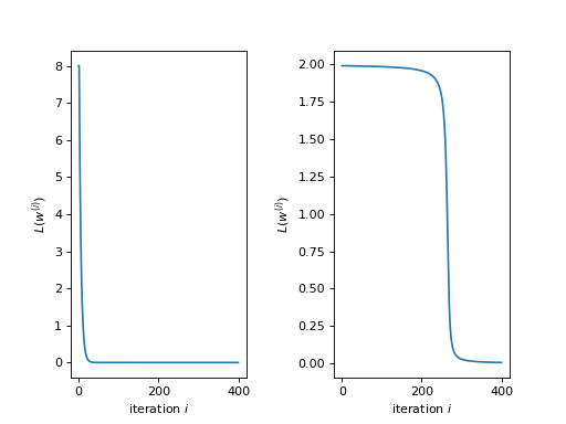
Both plots show the quadratic loss functions (12) per iteration of training of a linear (left) and a hyperbolic tangent (right) Adaline. Both started with an initial weight of $-3$ and were presented the signle training data element $(x^{(1)},y^{(i)})=(1,1)$ . The initial weight was chosen far off a reasonable value. Nevertheless, the linear Adaline learns to adjust the weight rather quickly while the hyperbolic tangent Adaline takes about more than two magnitudes more iteration before a significant learning progress can be observed.

For simplicity and to draw a nice connection to statistics, let us look at the logistic Adaline model, i.e., the Adaline model with $\alpha(z)$ being the logistic function (18). The same line of reasoning that will be developed for the logistic Adaline will apply to the hyperbolic tangent Adaline in the plot above.

Looking at our update rule (16) we can read off the explanation for the slow learning phenomenon. Recall the update rule:

$w \mapsto w^{\text{new}} := w + \eta \sum_{i=1}^M \left( y^{(i)}-\alpha(w\cdot x^{(i)}) \right) \alpha'(w\cdot x^{(i)}) x^{(i)}$

and the derivative of the logistic function (18):

(19)¶ $\alpha'(z) = \frac{e^{-z}}{(1+e^{-z})^2}=\alpha(z)(1-\alpha(z)).$

Clearly, for large values of $z$ the derivative $\alpha'(z)$ becomes very small, and hence, the update computed by the update rule (16) will be accordingly small even for the case of a misclassification. This is why this phenomenon is usually referred to as vanishig gradient problem.

If, for whatever reason, we would like to stick with the logistic function as activation function we can only try to adapt the loss function $L(w)$ in order to better the situation. How can this be done? Let us restrict our consideration to loss functions of the form

(20)¶ $L(w) = \sum_{i=1}^M l(y^{(i)},\alpha(w\cdot x^{(i)});$

note that with

(21)¶ $l(y,x) := \frac12 (y-x)^2$

the form (20) reproduces exactly the form of the quadratic loss function given in (12). We compute

(22)¶ $\frac{\partial L(w)}{\partial w} = \sum_{i=1}^M \frac{\partial l}{\partial z}(y^{(i)},z) \big|_{z=\alpha(w\cdot x^{(i)})} \cdot \alpha'(w\cdot x^{(i)}) \, x^{(i)}.$

This means that the only choice to compensate a potential vanishing gradient due to $\alpha'$ is to choose a good function $l$ . Bluntly, this could be done by choosing $\frac{\partial l}{\partial z}(y^{(i)},z) \big|_{z=\alpha(w\cdot x^{(i)})}$ to be proportional to the inverse of $\alpha'(w\cdot x^{(i)})$ and then integrating it – hoping to find a useful loss function for the training objective. We will not follow this route this but make a detour and use this opportunity to motivate a good candidate of the loss function by ideas drawn from statistics. The direct way, however, makes up a good homework and stands for its own as it is independent of the heuristics.

For this purpose we introduce the concept of entropy and cross-entropy. We define:

Definition (Entropy) Given a discreet probability space $(\Omega,P)$ we define the so-called entropy by

$H(P) := \sum_{\omega \in \Omega} P(\omega) \, (-1)\, \log_2 P(\omega).$

Note that $P(\omega)\in[0,1]$ but the sum is to be understood as summing only over $\omega$ such that $P(\omega)>0$ . when excluding events of probability zero as they since they would not have to to be encoded anyway. Heuristically speaking, the entropy function $H(P)$ measures how many bits are on average necessary to encode an event. Say Alice and Bob want to distinguish a number of $|\Omega|=N$ events but only have a communication channel through which one bit per communication can be send. An encoding scheme that is able distinguish $N$ events but on average minimizes the number of communications between Alice and Bob would allocate small bit sequences for frequent events and longer ones for infrequent ones. The frequency of an event $\omega\in\Omega$ is is determined by $P(\omega)$ so that the best strategy to minimize the average number of bits per event is to to allocate for event $\omega$ a number of $-\log_2(P(\omega))$ bits.

Let us regard a three examples:

A fair coin: The corresponding probability space can be modelled by

$\Omega = \{0,1\}, \qquad \text{and} \qquad \forall \omega\in\Omega: \quad P(\Omega):=\frac{1}{2}$

so that we find

$H(P) = -\sum_{\omega\in\{0,1\}}P(\omega)(-1)\log_2(P(\omega))=-\log_2\frac12 = 1.$

Hence, on average we need 1 bit to store the events as typically we have 0 or 1.
A fair six-sided dice: The corresponding probability space can be modelled by

$\Omega = \{1,2,3,4,5,6\}, \qquad \text{and} \qquad \forall \omega\in\Omega: \quad P_\text{fair}(\omega):=\frac{1}{6}$

and we find

$H(P_\text{fair}) = \sum_{\omega\in\{1,2,3,4,5,6\}}P(\omega)(-1)\log_2(P(\omega)) = -\log_2\frac{1}{6} \approx 2.58\ldots.$

Hence, on average we need 3 bits to store which of the six typical events occurred.
An unfair six-sided dice: Let us take again $\Omega=\{1,2,3,4,5,6\}$ but instead of the uniform distribution like above we chose:

$\omega$ $1$ $2$ $3$ $4$ $5$ $6$

$P_\text{unfair}(\omega)$ $1/4$ $1/16$ $1/16$ $1/16$ $1/16$ $1/2$

In this case we find

$H(P_\text{unfair}) = \sum_{\omega\in\{1,2,3,4,5,6\}}P(\omega)(-1)\log_2(P(\omega)) = -\log_2\frac{1}{6}= 2$

Since typically event $\omega=6$ occurs more often then the others we may afford to allocate less bits to represent it. The price to pay is to allocate more bits for the less frequent events. However, weighting with the relative frequency, i.e., on average, such an allocation turns out to require less bits per event to be transmitted through Alice and Bob’s communication channel. In particular, on average, they need less bits than in the case of the fair dice.

In statistics the actual probability measure $P$ is usually unknown and the objective is to find a good estimate $Q$ of it taking in account the empirical evidence. A candidate for a measure of how good such a guess is is given by the so-called cross-entropy which we define now.

Definition (Entropy) Given a discreet probability space $(\Omega,P)$ and another measure $Q$ we define the so-called cross-entropy by

$H(P,Q) := \sum_{\omega \in \Omega} P(\omega) \, (-1)\, \log_2 Q(\omega).$

One may interpret $H(P,Q)$ as follows: If $Q$ is an estimate of the actual probability measure then $-\log_2 Q(\omega)$ is the number of bits necessary to encode the event $\omega$ according to this estimate. The cross-entropy $H(P,Q)$ is therefore an average w.r.t. to the actual measure $P$ of the number of bits needed to encode the events $\omega\in\Omega$ according to $Q$ . If according to $Q$ we would allocate the wrong amount of bits to encode the events Alice and Bob would on average have to exchange more bits per communication. This indicates that $H(P,P)=H(P)$ must be the optimum which is actual:

Theorem (Cross-Entropy) Let $(\Omega,P)$ be a discreet probability space and $Q$ another measure on $\Omega$ . Then we have:

$H(P,Q) \geq H(P,P).$

Prove the theorem. Hint: Consider first the case of only two possible events, i.e., $|\Omega|=2$ and find the global minimum.

This property qualifies $H(P,Q)$ as a kind of distance between a potential guess $Q$ of the true probability $P$ . After this excursion to statistics let us employ this distance and with it build a loss function for the logistic Adaline by the following analogy.

For the logistic Adaline we assume the labels for features $x^{(i)}$ to be of the form $y^{(i)}\in\{0,1\}$ , $1\leq i\leq M$ . Furthermore, we observe that by definition also the activation functions evaluate to $\alpha(w\cdot x^{(i)})\in(0,1)$ . This allows to define for the sample space

$\Omega=\left\{\,\{x^{(i)} \text{ drawn and label is } 1\}\, \,\big|\,1\leq i\leq M\right\} \bigcup\left\{\,\{x^{(i)} \text{ drawn and label is } 0\}\, \,\big|\,1\leq i\leq M\right\}$

and the following probability distributions, i.e., the actual one (assuming the training data was labeled correctly and the $x^{(i)}$ are drawn with a uniform distribution),

$P(\{x^{(i)} \text{ drawn and label is } 1\}) & = \frac{y^{(i)}}{M} \\ P(\{x^{(i)} \text{ drawn and label is } 0\}) &= \frac{1-y^{(i)}}{M}$

and the neuron’s guess (which for sake of the probabilistic analogy we interpret as a probability),

$Q(\{x^{(i)} \text{ drawn and label is } 1\}) &= \frac{\alpha(w\cdot x^{(i)})}{M} \\ Q(\{x^{(i)} \text{ drawn and label is } 0\}) &=\frac{1-\alpha(w\cdot x^{(i)})}{M}.$

In order to measure the discrepancy between the actual measure $P$ and the guess $Q$ we employ the cross-entropy, which in our case, is defined as

$H(P,Q) &= \sum_{\omega\in\Omega} P(\omega)\log_2 Q(\omega)\\ &= \frac{1}{\log 2} \left( 1-\frac{1}{M} \sum_{i=1}^M \left( y^{(i)} \log(\alpha(w\cdot x^{(i)}) +(1-y^{(i)}) \log(1-\alpha(w\cdot x^{(i)}) \right) \right).$

Dropping the irrelevant constants we may define a new loss function $L(w)$ by using the following expression for (20)

(23)¶ $l(y, \alpha(w\cdot x)) := y \log(\alpha(w\cdot x) +(1-y) \log(1-\alpha(w\cdot x)$

so that we get

$L(w)= -\frac{1}{M} \sum_{i=1}^M \left( y^{(i)} \log(\alpha(w\cdot x^{(i)}) +(1-y^{(i)}) \log(1-\alpha(w\cdot x^{(i)}) \right).$

Using (19) we compute the derivative

$\frac{\partial L(w)}{\partial w} &= -\sum_{i=1}^M \left( \frac{y^{(i)}}{\alpha(w\cdot x^{(i)})} -\frac{1-y^{(i)}}{1-\alpha(w\cdot x^{(i)})} \right) \alpha'(w\cdot x^{(i)})\, x^{(i)}\\ &= -\left( \frac{y^{(i)}}{\alpha(w\cdot x^{(i)})} -\frac{1-y^{(i)}}{1-\alpha(w\cdot x^{(i)})} \right) \alpha(w\cdot x^{(i)})(1-\alpha(w\cdot x^{(i)}))\, x^{(i)}\\ &= \sum_{i=1}^M \left( \alpha(w\cdot x^{(i)})-y^{(i)} \right)\,x^{(i)}.$

We observe, that the vanishing gradient behavior of $\alpha'$ is compensated by the derivative of the cross-entropy $l'$ . In conclusion, we find the update rule corresponding to this new loss function

$w \mapsto w^{\text{new}} := w + \eta \sum_{i=1}^M \left( \alpha(w\cdot x^{(i)})-y^{(i)} x^{(i)} \right).$

A comparison with the previous update rule (22) shows that with the help of a change of loss function we end up with a update rule that will not show the vanishing gradient problem. As a rule of thumb one can expect that logistic Adalines will almost always be easier to train with cross entropy loss functions unless the vanishing gradient effect is desired – at a later point we may come back to this point and discuss that, e.g., in convolution networks the ReLu activation function (being zero for negative arguments and linear for positive ones) have actually proven to be very convenient. For now the take away from this section is that the choices in $\alpha(z)$ and $L(w)$ must be carefully tuned w.r.t. each other.

Adapt our Adaline implemetation with the logistic activation function and replace the old loss function by the cross-entropy and compare the learning behavior in both cases.

Support Vector Machine¶

While the Adaline loss functions (20) for the quadratic loss (21) or cross-entropy loss (23) were good measures of how accurately the training data is classified that can be used for optimization in terms of gradient descent, they did not put a particular emphasis on how the optimal weights $w$ may lead to a good generalization from the classification of “seen” training data to “unseen” data we may want to classify in the future. In the next model we shall specify such a sense and derive a corresponding loss function.

Hard Margin Case¶

Consider a typical linear separable case of training data. Depending on the initial weights both, the Adaline and Perceptron, may find separating hyperplanes of the same training data, however, the hyperplanes are usually not unique. Among all possible hyperplanes it may make sense to choose the one that maximizes the margin width as, e.g., shown in Figure Fig. 6.

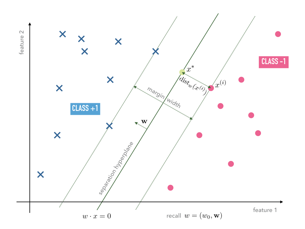
Fig. 6 Linear separable data with a separating hyperplane that maximizes the margin width.

In order to set up an optimization program that maximizes the margin width, let us compute the distance between a data point $x^{(i)}=(1,\mathbf x^{(i)})$ and the hyperplane $w=(w^0,\mathbf w)$ . For this purpose we exploit that the vector $\mathbf w$ is the normal vector on the plane. Hence, the straight line in direction of the normal vector $\mathbf w$ through the point $\mathbf x^{(i)}$ may be parametrized as follows

(24)¶ $x:\mathbb R\to\mathbb R^{n+1}, \qquad x(\alpha):= x^{(i)} + \alpha \begin{pmatrix} 0\\ \mathbf w \end{pmatrix} .$

Recall again that the first coefficient in the $\mathbb R^{n+1}$ vector was chosen to remain equal one by our convention. Furthermore, by definition, all points $x^*$ on the hyperplane $w$ fulfill

$w\cdot x^* = 0.$

Hence, we have to solve the equation

$0 = w\cdot (1,\mathbf x(\alpha)) = w^0 + \mathbf w\cdot\mathbf x^{(i)} + \alpha\,\mathbf w^2 = w\cdot x^{(i)} + \alpha\,\|\mathbf w\|^2$

for $\alpha$ in order to compute the intersection point $x^*$ between the straight line (24) and the hyperplane $w$ :

$x^*= x(\alpha) \qquad\text{for}\qquad \alpha = - \frac{w\cdot x^{(i)}}{\|\mathbf w\|^2}.$

The distance can then be computed by taking the difference

$\operatorname{dist_w}(x) := \|x^{(i)}-x^*\|$

which results in

$\operatorname{dist_w}(x^{(i)}) = \left\| \alpha \begin{pmatrix} 0\\ \mathbf w\end{pmatrix} \right\| = \frac{|w\cdot x^{(i)}|}{\|\mathbf w\|}.$

Any optimization program should, hence, choose a hyperplane $w$ that classifies the data points correctly according to their labels $y^{(i)}$ while trying to maximize the distance $\operatorname{dist_w}(x^{(j)})$ for such $j$ whose corresponding data points $x^{(j)}$ lie within minimal distance to the hyperplane – such points will in the following be called support vectors, hence, the name support vector machine. In order to make this notion precise without complicating the equations, we may exploit the scale invariance of the hyperplane equation $w\cdot x=0$ which may be build into the norm of $w$ and simply define the minimal distance between the nearest data points $x^{(i)}$ to the hyperplane $w$ equal to one so that all other distances are measured in this unit.

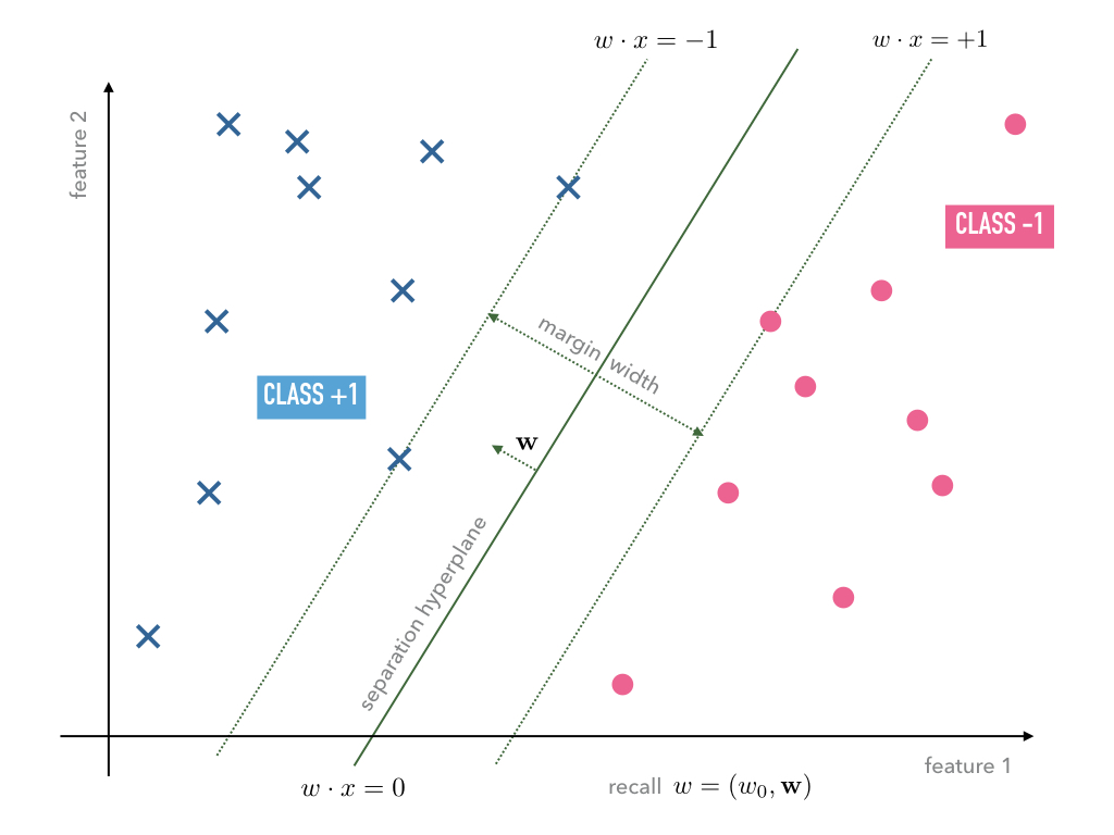
Fig. 7 With a weight vector $w$ on a scale such that the margin width equals $2$ .

On that scale, support vectors $x^{(j)}$ fulfill

$w\cdot x^{(j)} = \pm 1$

so that

$\operatorname{dist_w}(x^{(j)}) = \|\mathbf w\|^{-1}.$

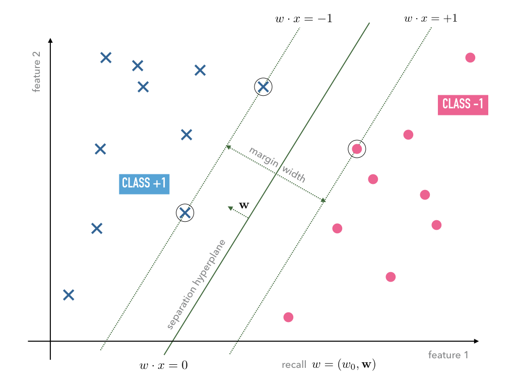
Fig. 8 The circled data points denote the support vectors.

Using this, we can formulate the constraints as we must require that the distance of any data point $x^{(i)}$ to the respective hyperplane $w\cdot x^{(i)}=y^{(i)}$ is larger or equal one. Hence, we may formulate the optimization program as

$\underset{w\in\mathbb R^{n+1}}{\text{maximize}} \quad \|\mathbf w\|^{-1} \qquad \text{subject to} \qquad \begin{cases} y^{(i)}\, w\cdot x^{(i)} \geq 1 \\ \text{for } 1\leq i\leq M \end{cases} .$

If we prefer, this program is equivalent to

(25)¶ $\underset{w\in\mathbb R^{n+1}}{\text{minimize}} \quad \|\mathbf w\| \qquad \text{subject to} \qquad \begin{cases} y^{(i)}\, w\cdot x^{(i)} \geq 1 \\ \text{for } 1\leq i\leq M \end{cases} .$

Note that the type of optimization is different to the one we have employed for the Adaline since now we need obey certain constraints during the optimization. Before we get to an implementation let us regard a useful generalization of this so-called hard margin case in which we do not allow any violation of the margin width.

Soft Margin Case¶

The optimization program (25) is very dependent on the fluctuation of data points near the margin. Possible outliers in the training data near or within the margin dictate how the “optimal” weights $w$ have to be chosen. To reduce this dependency we shall extend the hard margin program to the so-called soft-margin program as follows.

Let us in general allow margin violations but include in the optimization program that those have to be minimized. Suppose $x^{(i)}$ violates the margin width. This means that either

$0\leq y^{(i)}\, w\cdot x^{(i)} \leq 1$ in which case it is only a margin violation but not a misclassification or
$y^{(i)}\, w\cdot x^{(i)} > 1$ in which case it is a margin violation that leads to a misclassification,

which are illustrated in the following Figure Fig. 9

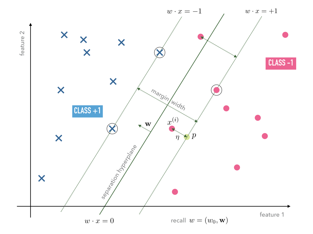
Fig. 9 Illustration of one misclassification and one simple margin violation.

The depth of a potential margin violation of data point $x^{(i)}$ can be computed following the same strategy as above. First, we compute the orthogonal projection $p$ of $x^{(i)}$ onto the hyperplane $w\cdot x=\pm 1$ as depicted in Figure Fig. 9, i.e., the point $p$ is given by the intersection of the straight line

$x:\mathbb R\to\mathbb R^{n+1}, \qquad x(\alpha):= x^{(i)} + \alpha \begin{pmatrix} 0\\ \mathbf w \end{pmatrix}$

and the hyperplane

$w\cdot x = y^{(i)}$

since the label $y^{(i)}$ determined the sign on the right-hand side. Hence, we have to solve the equation

$w\cdot x(\alpha) = y^{(i)}$

for $\alpha$ which gives

$\alpha = \frac{|y^{(i)} - w\cdot x^{(i)}|}{\|\mathbf w\|^2} = \frac{|1 - y^{(i)}\,w\cdot x^{(i)}|}{\|\mathbf w\|^2}.$

The depth of the margin violation is then given by the distance

$\eta^{(i)} = \|p - x^{(i)}\|=\frac{|1 - y^{(i)}\,w\cdot x^{(i)}|}{\|\mathbf w\|}.$

In order to allow for margin violations but also minimize them, we may now set up the following optimization program

$\underset{w\in\mathbb R^{n+1},\xi^{(i)}\geq 0, 1\leq i \leq M}{\text{minimize}} \quad \|\mathbf w\| + \sum_{i=1}^M \eta^{(i)} \qquad \text{subject to} \qquad \begin{cases} y^{(i)}\, w\cdot x^{(i)} \geq 1 - \|\mathbf w\|\, \eta^{(i)} \\ \text{for } 1\leq i\leq M \end{cases} .$

If we now change the scale once more to units of $\|\mathbf w\|^{-1}$ the program can be stated equivalently as

(26)¶ $\underset{w\in\mathbb R^{n+1},\xi^{(i)}\geq 0, 1\leq i \leq M}{\text{minimize}} \quad \|\mathbf w\|^2 + \sum_{i=1}^M \xi^{(i)} \qquad \text{subject to} \qquad \begin{cases} y^{(i)}\, w\cdot x^{(i)} \geq 1 - \xi^{(i)} \\ \text{for } 1\leq i\leq M \end{cases} .$

Implementation¶

In order to arrive at our first, as it will turn out, naive, implementation of the support vector machine for the soft margin case, we need to implement a version of the optimization program (26) and we shall do so in the spirit of the Adaline model. Later we will see that this can be done much more elegantly by reformulating the optimization program.

For this purpose we need a loss function to mimic the behavior of the program (26). A good candidate for this is given by

(27)¶ $L(w) = \frac{1}{2}\|\mathbf w\|^2 + \frac{\mu}{M}\sum_{i=1}^M \max\{0, 1-y^{(i)}\,w\cdot x^{(i)}\},$

where $\max S$ denotes the maximum of a set $S$ , $\mu$ is a parameter that controls the weight with respect to which the minimization of $\|\mathbf w\|^2$ is prioritized over the minimization of the accumulative margin violation. The factor $\frac12$ is just decoration, of course, and only kept because you will see it in many textbooks.

We may now be tempted to readily apply a gradient descent algorithm in order to find optimal weights $w$ . However, we recall that for this we need $L(w)$ to be a differentiable function of $w$ and due to the $\max$ function this is not the case. Nevertheless, we can approximate the derivative by means of a suitable candidate of its subdifferential. For example, we may simple set approximate gradient to be

(28)¶ $\operatorname{grad}L(w) := \|\mathbf w\| - \frac{\mu}{M}\sum_{i=1}^M y^{(i)}\, x^{(i)} \, \max\{0, 1-y^{(i)}\,w\cdot x^{(i)}\}$

and use the update rule

$w\mapsto w^{\text{new}} := w - \eta \operatorname{grad} L(w)$

for some learning parameter $\eta\in\mathbb R^+$ . To render the implementation of the update rule more transparent let us first create a class of methods that performs the computation of the loss function (27) as well as the approximate gradient (28):

class LossSVM:

    def __init__(self, X_train, Y_train, mu=1.0):
    """
    Initialize the parameter `mu` which specifies the weighting
    between margin width and the distance to the support vectors, and
    furthermore, the training data `X_train` and `Y_train`.
    """

       self.mu_ = mu

       self.xi_ = X_train
       self.yi_ = Y_train

       return

    def val(self, w):
       """
       Computes a value of the loss function for a given weight vector.
       """

       self.margin = 1 - self.yi_ * ( np.dot(self.xi_, w[1:]) + w[0] )

       w_norm = 1/2 * np.sum( w[1:]**2 )
       margin_violations = np.where(self.margin >= 0, self.margin, 0)
       margin_avg = margin_violations.sum() / len(self.xi_)

       return w_norm + self.mu_ * margin_avg

    def diff(self, w):
       """
       Computes the derivative of the loss function for a given weight vector.
       """

       self.margin = 1 - self.yi_ * ( np.dot(self.xi_, w[1:]) + w[0] )

       w0_sub_diff1 = - self.yi_
       w0_sub_diffs = np.where(self.margin >= 0, w0_sub_diff1, 0)
       w0_diffs_avg = w0_sub_diffs.sum() / len(self.xi_)

       w_sub_diff1 = - self.xi_ * self.yi_[:,np.newaxis]
       w_sub_diffs = np.where(self.margin[:,np.newaxis] >= 0, w_sub_diff1, 0)
       w_diffs_avg = w_sub_diffs.sum(axis=0) / len(self.xi_)

       ret0 = np.array([ w0_diffs_avg ])
       ret_vec = w[1:] + self.mu_ * w_diffs_avg

       return np.append(ret0, ret_vec)

This class expects the training data as arguments X_train and Y_train in the constructor in line 3;
The val() method in line 15 determines the value of the loss function for the training data specified in the constructor;
Furthermore, the method diff() computes the approximate derivative stated in (28).

The rest of the implementation follows the Adline one except, of course, that the learning rule has to be replaced:

def learn(self, X_train, Y_train, mu=1.0, eta=0.01, epochs=1000):
    '''
    fit training data according to eta and n_iter
    and log the errors in errors_
    '''

    # we initialize two list, each for the misclassifications and the cost function
    self.train_errors_ = []
    self.train_loss_ = []

    # for all the epoch
    for _ in range(epochs):
        # classify the traning features
        Z = self.classify(X_train)
        # count the misqualifications for the logging
        err = 0
        for z, y in zip(Z, Y_train):
            err += int(z != y)
        # ans save them in the list for later use
        self.train_errors_.append(err)

        loss = LossSVM(X_train, Y_train, mu=mu)
        # compute loss for this epoch
        self.train_loss_.append( loss.val(self.w_) )
        # compute gradient of loss function and with it the update for w
        delta_w = - eta * loss.diff(self.w_)
        # update the weights
        self.w_ += delta_w

    return

The LossSVM class that we defined above is instantiated with loss in the main loop and the entire training data is passed to its constructor;
The computation of the loss function is carried out in line 24 while the update happens in line 26.

SOURCECODE: where_to_go/iris_svm.ipynb

The full implementation of the ‘naive’ version of the support vector machine.

SOURCECODE: where_to_go/iris_svm_convergence.ipynb

These are the same test scenarios that we used to observe the learning behavior for the Perceptron and Adaline.

Implement the support vector machine as mini-batch learner and play with the two parameters mu and eta in scenarios that feature margin violations in order to get a feeling about their influence.

First Non-Linear Classification¶

Todo

Under construction. See for example [13].

Rough notes: Non-linear extension of the Adaline

Multi-Class Classification¶

Todo

Under construction. See for example [13].

Rough notes: Multi-class extension of the Adaline

Where to go from here?¶

Sigmoid activation function¶

Support Vector Machine¶

Hard Margin Case¶

Soft Margin Case¶

Implementation¶

First Non-Linear Classification¶

Multi-Class Classification¶

Mathematics and Applications of Machine Learning

Navigation

Related Topics

$\omega$	$1$	$2$	$3$	$4$	$5$	$6$
$P_\text{unfair}(\omega)$	$1/4$	$1/16$	$1/16$	$1/16$	$1/16$	$1/2$