1 Version notes: 2016-08-15

As always, these notes have been written in quite a haste during the semester and will contain lots of typos. Many of them were already spotted and corrected by my students of the 2016 summer semester course at LMU, and I am particularly grateful for Pavel Fadeev’s help. If you still find a typo please help to improve these notes and report it with a precise reference (URL, equation number, etc.) to my email address above. To my students: This material is in most parts less detailed than the discussion in the lecture. Please let me know if and where, you feel the notes came too short. Thanks in advance!

2 Review: Vlasov-Maxwell equations

The previous lectures ended with the discussion of the informal limit \(\hbar\to 0\) of the transport equations of QED of a dilute gas of electrons when neglecting the spin term. In particular, we have found the so-called Vlasov-Maxwell equations, i.e., \(\eqref{eq:vlasov}, \eqref{eq:maxwell-one}, \eqref{eq:constraints-one}\) below, that describe the evolution of a phase space density \[ f:(\bb R,\bb R^3,\bb R^3)\to \bb R^+_0, \qquad (t,\vv q,\vv p) \mapsto f_t(\vv q,\vv p). \] The latter density provides a measure \(f_t(\vv q,\vv p)d^3q d^3p\) with respect to which we may compute expectation values. For instance, the expected charge density \(\rho_t\) and the current density \(\vv j_t\) are given by \[ \rho_t(\vv x) = e\int d^3p \, f_t(\vv x,\vv p), \qquad \vv j_t(\vv x) = e\int d^3p\, \vv v(\vv p) f_t(\vv x,\vv p), \] where \(e\) denotes the charge of an electron, by convention, having a negative sign. In the following we will use Gaussian units throughout our discussion.

We have found that the equation of motion obeyed by \(f_t(\vv q, \vv p)\) is the so-called Vlasov equation \[ \label{eq:vlasov} \partial f_t(\bb q,\bb p) = - \vv v(\vv p) \cdot \partial_{\vv q} f_t(\vv q,\vv p) - e\vv L(\vv q,\vv p,\vv E_t,\vv B_t) \cdot \partial_{\vv p} f_t(\vv q,\vv p), \] where \(\vv v(\vv p) = \frac{\vv p}{\sqrt{\vv p^2+m^2}}\) is the relativistic velocity and \[ \label{eq:lorentz-one} \vv L(\vv q,\vv p, \vv E, \vv B) = \vv E(\vv q) + \vv v(\vv p)\wedge \vv B(\vv q) \] is the Lorentz force. The electric and magnetic fields \(\vv E_t\) and \(\vv B_t\) are dynamical degrees of freedom of their own and satisfy the Maxwell equations \[ \label{eq:maxwell-one} \partial_t \begin{pmatrix} \mathbf E_{t} \\ \mathbf B_{t} \end{pmatrix} = \begin{pmatrix} \nabla \wedge \mathbf B_{t} - 4\pi \mathbf j_t \\ -\nabla \wedge \mathbf E_{t} \end{pmatrix} \] and the Maxwell constraints \[ \label{eq:constraints-one} \nabla\cdot \vv E_t(\vv x) = 4\pi \rho_t(\vv x), \qquad \nabla\cdot \vv B_t(\vv x) = 0 \] with respect to the expected charge densities \(\rho_t\) and currents \(\vv j_t\).

3 The equations of motion of classical electrodynamics

The system of PDEs \(\eqref{eq:vlasov}, \eqref{eq:maxwell-one}, \eqref{eq:constraints-one}\) of the Vlasov-Maxwell equations are intimately connected to the equation of motions of a cloud of \(N\in\bb N\) like charges having position \(t\mapsto\vv q_{i,t}\in\bb R^3\), momentum \(t\mapsto\vv p_{i,t}\in\bb R^3\), and labels \(i=1,\ldots,N\). The phase space density corresponding to such a gas of charges would take the form \[ \label{eq:cloud} f_t(\vv q,\vv p)=\sum_{i=1}^N \delta^3(\vv q-\vv q_{i,t}) \delta^3(\vv p-\vv p_{i,t}). \] Informally, for \(\eqref{eq:cloud}\) to be a solution of the Vlasov-Maxwell equations \(\eqref{eq:vlasov}, \eqref{eq:maxwell-one}, \eqref{eq:constraints-one}\) one finds – homework – that the charge trajectories \(t\mapsto(\vv q_{i,t},\vv p_{i,t})\) have to fulfill \[ \label{eq:lorentz-self} \frac{d}{dt} \begin{pmatrix} \vv q_{i,t}\\ \vv p_{i,t}\\ \end{pmatrix} = \begin{pmatrix} \vv v(\vv p_{i,t})\\ e \vv L(\vv q_{i,t},\vv p_{i,t}, \vv e_t,\vv b_t) \end{pmatrix} \] together with the expression for the Lorentz force \(\eqref{eq:lorentz-one}\), the Maxwell equations \[ \label{eq:maxwell-self} \partial_t \begin{pmatrix} \mathbf e_t \\ \mathbf b_t \end{pmatrix} = \begin{pmatrix} \nabla \wedge \mathbf b_t - 4\pi e \sum_{i=1}^N \vv v(\vv p_{i,t})\delta^3(\cdot-\vv q_{i,t}) \\ -\nabla \wedge \mathbf e_t \end{pmatrix}, \] and constraints \[ \label{eq:constraints-self} \nabla\cdot \vv e_t(\vv x) = 4\pi e \sum_{i=1}^N\delta^3(\vv x-\vv q_{i,t}), \qquad \nabla\cdot \vv b_t(\vv x) = 0. \]

3.1 The Coulomb or ultraviolet divergence

We emphasized “informally” not only because \(f_t\) is now a distribution but more to the point because the latter system of coupled ODEs and PDEs \(\eqref{eq:lorentz-self},\eqref{eq:maxwell-self}, \eqref{eq:constraints-self}\) is ill-defined as we shall see. This fact and the source of the problem can be seen best when splitting up the fields \(\vv e_t\) and \(\vv b_t\) into individual fields generated by each of the \(N\) charges. This can be done thanks to the linearity of the Maxwell equations \(\eqref{eq:maxwell-self}\) in the field degrees of freedom. The resulting systems of equations is: \[ \label{eq:lorentz-point} \frac{d}{dt} \begin{pmatrix} \vv q_{i,t}\\ \vv p_{i,t}\\ \end{pmatrix} = \begin{pmatrix} \vv v(\vv p_{i,t})\\ \sum_{j=1}^N e_{ij} \vv L(\vv q_{i,t}, \vv p_{i,t}, \vv e_{j,t},\vv b_{j,t}) \end{pmatrix}, \] \[ \label{eq:maxwell-point} \partial_t \begin{pmatrix} \mathbf e_{i,t} \\ \mathbf b_{i,t} \end{pmatrix} = \begin{pmatrix} \nabla \wedge \mathbf b_{i,t} - 4\pi e \vv v(\vv p_{i,t})\delta^3(\cdot-\vv q_{i,t}) \\ -\nabla \wedge \mathbf e_{i,t} \end{pmatrix}, \] \[ \label{eq:constraints-point} \nabla\cdot \vv e_{i,t}(\vv x) = 4\pi e \delta^3(\vv x-\vv q_{i,t}), \qquad \nabla\cdot \vv b_{i,t}(\vv x) = 0 \] for \(i=1,\ldots,N\). For the trivial matrix of coupling constants \(e_{ij} = e\) for \(i,j=1,\ldots,N\), the system of equations \(\eqref{eq:lorentz-point},\eqref{eq:maxwell-point},\eqref{eq:constraints-point}\) is equivalent to the one above \(\eqref{eq:lorentz-self},\eqref{eq:maxwell-self},\eqref{eq:constraints-self}\) setting \(\vv e_t=\sum_{i=1}^N \vv e_{i,t}\) and \(\vv b_t=\sum_{i=1}^N \vv b_{i,t}\). A general coupling matrix \(e_{ij}\) can be used to tune or switch on and off the interaction strength between the \(i\)th charge and the \(j\)th field which will be convenient for a later discussion. Note that due to \(\eqref{eq:constraints-point}\) we may interpret the \(i\)th field as generated by the \(i\)th charge.

The Maxwell equations and constraints \(\eqref{eq:maxwell-point},\eqref{eq:constraints-point}\) form an inhomogeneous system of linear PDEs. Hence, all its solutions can be found by choosing one of its solutions and adding solutions of the homogeneous equations (i.e., solutions to \(\eqref{eq:maxwell-point},\eqref{eq:constraints-point}\) for \(e=0\)). For a given charge trajectory \(t\mapsto(\vv q_t,\vv p_t)\), dropping the label \(i\) for a moment, two special inhomogeneous solution are known under the name retarded and advanced Liénard-Wiechert fields: \[ \begin{align} \definecolor{red}{RGB}{200,80,80} \vv e^{\pm}_t(\vv x) &:= \frac{({\vv n}\pm\vv v)(1-\vv v^2)} {{\color{red}|\vv x - \vv q|^2}(1\pm {\vv n}\cdot\vv v)^3} + \frac{{\vv n}\wedge[({\vv n}\pm\vv v)\wedge \vv a]}{|\vv x -\vv q|(1\pm {\vv n}\cdot\vv v)^3}\bigg|^\pm, \nonumber \\ \vv b^{\pm}_t(\vv x) &:= \mp \vv n^{\pm}\wedge\vv e^{\pm}_t(\vv x), \label{eq:lw} \end{align} \] where we have used the abbreviations \[ \begin{align} \label{eq:lw-abbreviations} \begin{array}{rlrlc} \vv q^\pm &:= \vv q_{t^\pm}, \qquad\mbox{} &\vv v^\pm &:= \vv v(\vv p_{t^\pm}), \qquad\mbox{} & \vv a^\pm := \frac{d}{dt}{\vv v}(\vv p_{t})\Big|_{t=t^{\pm}},\\ \vv n^\pm &:= \frac{\vv x-\vv q^\pm}{|\vv x-\vv q^\pm|}, & t^\pm &:= t \pm |\vv x-\vv q^\pm|; \end{array} \end{align} \] One can check by direct computation – homework – that the fields in \(\eqref{eq:lw}\) are solutions to the Maxwell equations and constraints \(\eqref{eq:maxwell-point},\eqref{eq:constraints-point}\), respectively. Now, taking a closer look at the red denominator in \(\eqref{eq:lw}\) reveals that, e.g., \(\vv e_t\) has a pole of second order everywhere on the charge trajectory \(t\mapsto \vv q_{i,t}\); note that the delayed time \(t^\pm\) converges to \(t\) as \(\vv x\) approaches \(\vv q_t\). This singularity is often referred to as “Coulomb singularity”.

As explained above, we may now represent any solutions of the inhomogeneous equations \(\eqref{eq:maxwell-self},\eqref{eq:constraints-self}\) in terms of the sum \[ f_t = \lambda f^-_t[\vv q,\vv p] + (1-\lambda) f^+_t[\vv q,\vv p] + f^0_t, \] for \(\lambda\in[0,1]\) and \(f^\pm_t[\vv q,\vv p]=(\vv e_t^\pm,\vv b^\pm_t)\) denoting the retarded and advanced Liénard-Wiechert fields \(\eqref{eq:lw}\) above – the square brackets emphasize the functional dependence on the entire charge trajectory \(t\mapsto(\vv q_t,\vv p_t)\). Furthermore, \(f^0_t\) denotes a solution to the homogeneous Maxwell equations and constraints, i.e., \(\eqref{eq:maxwell-point},\eqref{eq:constraints-point}\) for \(e=0\). The latter cannot cancel the second order pole of \(f_t^\pm\), and thus, every solution \(f_t=(\vv e_t,\vv b_t)\) of the Maxwell equations and constraints \(\eqref{eq:maxwell-point},\eqref{eq:constraints-point}\) will exhibit the Coulomb singularity.

In consequence, the terms \(\vv L(\vv q_{i,t},\vv p_{i,t},\vv e_{j,t},\vv b_{j,t})\) for \(j=i\) are ill-defined and the system of equations \(\eqref{eq:lorentz-point},\eqref{eq:maxwell-point},\eqref{eq:constraints-point}\) does not make mathematical sense. In this notation the source of the problem can be interpreted as follows: The back reaction of the \(i\)th field generated by the \(i\)th charge is ill-defined – homework.

3.2 Rigid charges

In order to proceed somehow, we introduce a smearing of the point-charges by a rigid charge distribution \(\rho\in\cc C^\infty_c(\bb R^3,\bb R)\) as we have done in our quantum field theory toy model. More precisely, we replace the point-charge fields \(\vv e_{i,t},\vv b_{i,t}\) by the expressions \[ \vv E_{i,t} = \rho * \vv e_{i,t}, \qquad \vv B_{i,t} = \rho * \vv b_{i,t}, \] where \(*\) denotes the convolution. Note that the fields \(\vv E_{i,t}\) and \(\vv B_{i,t}\) behave much better because for \(|\vv x-\vv q_{i,t}|\to 0\) the expression \[ \begin{align} \vv E_{i,t}(\vv x) = \rho * \vv e_{i,t}(\vv x) &= \int d^3y \, \rho(\vv x-\vv y) O_{|\vv x-\vv q_{i,t}|\to 0}(|\vv y-\vv q_{i,t}|^{-2})\\ &= \int d^3z \, \rho(\vv x-\vv q_{i,t}-\vv z) O_{|\vv z|\to 0}(|\vv z|^{-2})\\ &= \int d\Omega\int_0^\infty dz \, \rho(\vv x-\vv q_{i,t}-\vv z) |z|^2 O_{|\vv z|\to 0}(|\vv z|^{-2}) \end{align} \] remains well-defined.

The above prescription turns our equations of motion into \[ \label{eq:lorentz-rho} \frac{d}{dt} \begin{pmatrix} \vv q_{i,t}\\ \vv p_{i,t}\\ \end{pmatrix} = \begin{pmatrix} \vv v(\vv p_{i,t})\\ \sum_{j=1}^N e_{ij} \int d^3x \, \rho(\vv x-\vv q_{i,t}) \left( \vv E_{j,t}(\vv x) + \vv v(\vv p_{i,t})\wedge \vv B_{j,t}(\vv x) \right) \end{pmatrix}, \] \[ \label{eq:maxwell-rho} \partial_t \begin{pmatrix} \mathbf E_{i,t} \\ \mathbf B_{i,t} \end{pmatrix} = \begin{pmatrix} \nabla \wedge \mathbf B_{i,t} - 4\pi e \vv v(\vv p_{i,t})\rho(\cdot-\vv q_{i,t}) \\ -\nabla \wedge \mathbf E_{i,t} \end{pmatrix}, \] \[ \label{eq:constraints-rho} \nabla\cdot \vv E_{i,t}(\vv x) = 4\pi e \rho(\vv x-\vv q_{i,t}), \qquad \nabla\cdot \vv B_{i,t}(\vv x) = 0, \] where for reasons of symmetry we have also smeared out the Lorentz force in \(\eqref{eq:lorentz-rho}\). Hence, the form factor \(\rho\) can be interpreted as rigid geometrical extend of each charge. These system of equations has now a fighting chance to admit a well-posed initial value problem, which we shall discuss next.

3.3 Existence of dynamics for rigid charges

To compress the notation it is useful to recast \(\eqref{eq:lorentz-rho}, \eqref{eq:maxwell-rho}\) into the form \[ \begin{align} \label{eq:ml} \partial_t \varphi_t = A \varphi_t + J(\varphi_t). \end{align} \] Here, we have set \(\varphi_t=(\vv q_{i,t},\vv p_{i,t},\vv E_{i,t},\vv B_{i,t})_{i=1,\ldots, N}\) and \(A\) and \(J\) informally act according to \[ \begin{align} A\varphi &= (0,0,\nabla\wedge \vv B_{i,t},-\nabla\wedge\vv E_{i,t})_{i=1,\ldots, N},\\ J(\varphi) &=\Big(\vv v(\vv p_{i}),\sum_{j=1}^N e_{ij} \int d^3x \, \rho(\vv x-\vv q_{i}) \left( \vv E_{j}(\vv x) + \vv v(\vv p_{i})\wedge \vv B_{j}(\vv x)\right), \\ & \qquad \qquad\qquad \qquad\qquad \qquad\qquad \qquad -4\pi e\vv v(\vv p_i)\rho(\cdot-\vv q_i), 0 \Big)_{i=1,\ldots, N}, \end{align} \] for \(\varphi=(\vv q_{i},\vv p_{i},\vv E_{i}\vv B_{i})_{i=1,\ldots, N}\).

This choice is motivated by the conserved energy of the homogeneous Maxwell equation and furthermore by the helpful Hilbert space structure. The differential operator \(A\) is then defined on its natural domain \[ D(A)=\left\{\varphi \in\cc H \,\big|\, A\varphi \in \cc H \right\}. \] whereas \(J\) maps any vector \(\varphi\in\cc H\) into \(\bigcap_{n=0}^\infty D(A^n)\) as \(\rho\) is smooth and compactly supported.

4 The point-charge limit

From a fundamental perspective, the form factor \(\rho\) is unwanted for several reasons, maybe most crucially:

• it introduces an additional and seemingly arbitrary (see remark below) parameter in our theory;
• it breaks relativistic invariance (even when \(\rho\) is correctly boosted).
• to date an electron does not seem to have an inner structure – not to mention classically;

Early on, Abraham recognized the point-charge problem and many others, such as Sommerfeld, Fokker, Schwarzschild, Tetrode, Dirac, Born, Infeld, Synge, Wheeler, Feynman, Landau, and Lifschitz, attempted formulations of classical electrodynamics of point-charges. In fact, in the beginning of the last century it was one of the most fashionable topics in mathematical physics. Despite the many efforts it remains an open problem. It was of course understood that at the scale of elementary particles (such as the electron) classical theory will fail, but nevertheless it is fair to ask whether classical electrodynamics allows for a relativistic formulation or not – especially when quantum field theory is plagued by the same ultraviolet problem, as we have discussed in part 1, which has yet prevented a formulation of an equation of motion.

Regarding the ill-defined equation of motion \(\eqref{eq:lorentz-self},\eqref{eq:maxwell-self},\eqref{eq:constraints-self}\) one may take at least two different positions (unless one is inclined to reformulate the whole theory):

1. The Lorentz equations \(\eqref{eq:lorentz-self}\) are wrong;
2. The Maxwell equations \(\eqref{eq:maxwell-self},\eqref{eq:constraints-self}\) are wrong.

Famous attempts regarding 1. are the mass-renormalization method proposed by Dirac and the action-at-a-distance formulation of Fokker, Schwarzschild, Tetrode and later Wheeler and Feynman, while for instance Born and Infeld took up route 2. and replaced the Maxwell equations by a non-linear version. As yet none of the attempts are entirely satisfying or mathematically sufficiently understood. Here we shall briefly discuss Dirac’s famous paper (Dirac 1938) that introduced the concept of “mass renormalization” which later inspired many renormalization methods that are still employed in modern quantum field theory.

Dirac’s starting point was to trust the Maxwell equations \(\eqref{eq:maxwell-self},\eqref{eq:constraints-self}\) and search for an equation of motion of the charges that would replace the ill-defined \(\eqref{eq:lorentz-self}\). In the following discussion we will at first restrict us to the case of only one charge interacting with its own and an additional external field (which drives the particle). Employing relativistic notation, we denote the world line of the charge by \(\tau\mapsto z^\mu(\tau)\). The Maxwell equations and constraints of the field tensor \(F^{\mu\nu}\) generated by this charge can then be cast into the form \[ \partial_\nu F^{\mu\nu}(x) = 4\pi e j^\mu(x), \quad \partial_\alpha\epsilon^{\alpha\beta\gamma\delta}F_{\gamma\delta} = 0 \] give the charge current \[ j^\mu(x)=\int_{\tau\mapsto z^\mu(\tau)} dz\, \delta^4(x-z). \] As discussed above, the field tensor \(F\) can be split up in the following contributions \[ \label{eq:field-splitting} F_+ + F_{out} + F_{ext} = F = F_- + F_{in} + F_{ext}, \] where \(F_\pm\) denote the corresponding Liénard-Wiechert fields of the world line \(\tau\mapsto z^\mu(\tau)\) (see homework above) and \(F_{in}\), \(F_{out}\), and \(F_{ext}\) denote the free incoming, free outgoing, and external field. Equation \(\eqref{eq:field-splitting}\) should be read as a definition of \(F_{in}\) and \(F_{out}\).

It is reasonable to assume that the equation of motion of the charge to be found should allow for some sense of energy-momentum conservation between the field and the charge degrees of freedom. To get information about the energy-momentum flux in the vicinity of a world-line one may compute the surface integral over the energy-momentum tensor \[ 4\pi {T^\mu}_\nu= F^{\mu\alpha} F_{\alpha\nu} + \frac14 g^{\mu\nu} F^{\alpha\beta} F_{\alpha\beta} \] of a tube \(\bb T\) with radius \(\epsilon>0\) around the \([\tau_1,\tau_2]\) interval of the world-line \(\tau\mapsto z^\mu(\tau)\), i.e., \[ \label{eq:energy-momentum-loss} \int_{\partial \bb T(\tau_1,\tau_2)} n_\mu(x) T^{\mu\nu}(x) d\sigma(x). \] Dirac argued that this quantity does only depend on \(\tau_1\) and \(\tau_2\) since replacing \(\bb T\) by another surface \(\bb T'\) would only result in an additional surface integral \[ \int_{vol(\bb T,\bb T')} \partial_\mu T^{\mu\nu}(x) d^4x \] which vanishes because \[ \label{eq:conservation-law} \partial_\mu T^{\mu\nu}(x) = 4\pi F^{\nu\mu}(x)j_\mu(x) \] is zero as the current has no support in \(vol(\bb T,\bb T')\) – homework.

For his computation, Dirac chose a tube of constant radius \(\epsilon\) perpendicular to the four-velocity \(\dot z^\mu(\tau)\) and expanded the Liénard-Wiechert fields \(F_\pm\) on this surface by means of a Taylor series in terms of radius \(\epsilon\) (in a rather lengthy computation which we will not repeat here). Neglecting higher order in \(\epsilon\) he found \[ \label{eq:energy-dirac} (\ref{eq:energy-momentum-loss}) = \int_{\tau_1}^{\tau_2} d\tau \left(-\frac{e^2}{2\epsilon} \ddot z^\nu(\tau) + e f^{\nu\mu}(z(\tau))\dot z_\mu(\tau)\right), \] where \[ \label{eq:little-f} f = F - \frac12 (F_-+F_+ ). \] The divergence on the right-hand side of \(\eqref{eq:energy-dirac}\) for \(\epsilon\to 0\) is due to the Coulomb singularity of the fields already observed above, and therefore, not surprising. As \(\eqref{eq:energy-dirac}\) may only depend of \(\tau_1\) and \(\tau_2\) we have \[ \label{eq:kin-energy} (\ref{eq:energy-momentum-loss}) = (\ref{eq:energy-dirac}) = P^\nu(\tau_2)-P^\nu(\tau_1) \] for \[ \label{eq:pdot} \dot P^\nu(\tau) = -\frac{e^2}{2\epsilon} \ddot z^\nu(\tau) + e f^{\nu\mu}(z(\tau))\dot z_\mu(\tau). \] Recall that the law which \(z^\nu(\tau)\) obeys is unknown and the goal is to find a good candidate. Equation \(\eqref{eq:pdot}\) however leaves a lot of possible candidates for \(P^\nu(\tau)\). Nevertheless, due to translational invariance, \(P^\nu\) may only depend of the four-velocity and its derivatives, Dirac argues that the ansatz \[ \label{eq:guess} P^\nu = m \dot z^\nu \] for some constant \(m\) is probably the simplest – homework:

First, because of \(\dot P^\nu(\tau) \dot z_\nu(\tau) = 0\), it yields a relativistic force law, and second, it allows to interpret the right-hand side of \(\eqref{eq:kin-energy}\) as difference of four-momenta. Hence, \(\eqref{eq:kin-energy}\) already states the energy-momentum conservation between the charge and field degrees of freedom.

In order to carry out the limit \(\epsilon\to 0\), Dirac suggests to absorb the mentioned divergence into the unknown parameter \(m\) by rescaling it such that \[ \label{eq:mass-ren} m_{ren} = m+\frac{e^2}{2\epsilon} \] remains constant. Of course, this implies that \(m\) has to be a function of \(\epsilon\) and then yields the equation \[ m_{ren} \ddot z^\nu(\tau) = e f^{\nu\mu}(z(\tau))\dot z_\mu(\tau), \] which must be obeyed by the charge world line \(\tau\mapsto z^\nu(\tau)\). In order to infer an initial value problem one may recast the auxiliary field in terms of \[ f = \frac12(F_{-}-F_{+}) + F_{in} + F_{ext} \] using \(\eqref{eq:field-splitting}\) and \(\eqref{eq:little-f}\). The Taylor expansion in \(\epsilon\) that has been used before, one now finds \[ \label{eq:radiation-reaction} \frac12(F^{\nu\mu}_{-}-F^{\nu\mu}_{+}) = e\frac{2}{3}(\dddot z^\nu \dot z^\nu + \dddot z^\nu\dot z^\mu) \] in the vicinity of the world line (neglecting all higher orders in \(\epsilon\)) so that the equation of motion for the charge takes the form \[ \label{eq:lad} m_{ren} \ddot z^\nu(\tau) = e^2\frac{2}{3}(\dddot z^\nu(\tau) \dot z^\nu(\tau) + \dddot z^\nu(\tau)\dot z^\mu(\tau)) + e (F_{in}+F_{ext})^{\nu\mu}(z(\tau))\dot z_\mu(\tau) \] This is the so-called Lorentz-Abraham-Dirac equation (LAD equation) and the first term on the right-hand side is usually referred to as ‘radiation reaction’ or ‘radiation friction’ term. As we shall see, it is a third order ODE with a well-posed initial value problem, i.e., each prescribed tuple \((z^\nu(0),\dot z^\nu(0),\ddot z^\nu(0)\) identifies a unique solution.

The argument above can be extended effortlessly to \(N\) charges with world lines \(\tau\mapsto z_i^\mu(\tau)\) and fields \(F_i=F_{in, i}+F_{-,i}\): \[ \begin{align} m_{ren} \ddot z_i^\nu = & e^2\frac{2}{3}(\dddot z_i^\nu \dot z_i^\nu + \dddot z^\nu_i\dot z_i^\mu) \dot z_{i,\mu} \\ &+ e \left(F_{in,i}+F_{ext} + \sum_{j\neq i}^N ( F_{in,j}+F_{-,j})\right)^{\nu\mu}(z_i)\dot z_{i,\mu} \end{align} \] for \(i=1,\dots,N\). The terms on the right-hand side then describe the radiation reaction, the interaction with the \(i\)th incoming field and the external field, and the \(j\neq i\) incoming and retarded fields of all the other charges.

4.1 Solutions of the LAD equation

For the sake of brevity and wherever unambiguous we will use the notations \(a\cdot b= a_\mu b^\mu\), \(a^2=a\cdot a\) for four-vectors \(a^\mu\), do not make the \(\tau\) dependence explicit, and, forgetting the mass renormalization procedure for a short while, also drop the subscript “ren” of the mass term \(m_{ren}\).

4.1.1 Case: No incoming or external field

We start with equation \(\eqref{eq:lad}\) and use the relations \[ z^2 = 1 \Rightarrow\ddot z\cdot \dot z = 0 \Rightarrow \dddot z\cdot \dot z = -\ddot z^2 \] to recast \(\eqref{eq:lad}\) as \[ \label{eq:LAD-short} \ddot z^\mu = \tau_0 (\dddot z^\mu + \ddot z^2 \dot z^\mu), \] where \(\tau_0=\frac{2e^2}{3m}\). Contracting this equation with \(\ddot z_\mu\) and rewriting the right-hand side in terms of a derivative gives \[ \ddot z^2 = \frac{\tau_0}{2} \frac{d}{d\tau} \ddot z^2. \] The well-known solution to this equation is \[ \label{eq:square-sol} \ddot z^2 = -A^2 e^{2\tau/\tau_0} \] for initial value \[ \label{eq:A} A=\sqrt{-\ddot z(0)^2}. \] Note that the relativistic acceleration is always non-positive – homework.

The observation \(\eqref{eq:square-sol}\) implies \[ \ddot z^\mu = \tau_0 (\dddot z^\mu -A^2 e^{2\tau/\tau_0} \dot z^\mu) \] which can again be solved by elementary methods. The general solution takes the form \[ \label{eq:sol-vel} \dot z^\mu = B_1^\mu \cosh(\tau_0 A e^{\tau/\tau_0}) + B_2^\mu \sinh(\tau_0 A e^{\tau/\tau_0}) \] which is parametrized by the initial data \(A\) in \(\eqref{eq:A}\) as well as by the following constants \(B_1^\mu\) and \(B_2^\mu\): \[ \begin{align} \label{eq:B} B_1^\mu &= \dot z^\mu(0) \cosh(\tau_0 A) - \frac{\ddot z^\mu(0)}{A} \sinh(\tau_0 A), \\ B_2^\mu &= -\dot z^\mu(0) \sinh(\tau_0 A) + \frac{\ddot z^\mu(0)}{A} \cosh(\tau_0 A). \end{align} \] For the discussion also the corresponding acceleration will be of interest: \[ \label{eq:sol-accel} \ddot z^\mu = B_1^\mu A e^{\tau/\tau_0}\sinh(\tau_0 A e^{\tau/\tau_0}) + B_2^\mu A e^{\tau/\tau_0}\cosh(\tau_0 A e^{\tau/\tau_0}) \]

To get acquainted to these solutions, let us make the following first observations:

1. As expected for a third order ODE, we observe that every solution \(\tau \mapsto z^\mu(\tau)\) to \(\eqref{eq:LAD-short}\) is uniquely parametrized by the initial data \((z^\mu(0),\dot z^\mu(0),\ddot z^\mu(0))\) since \(A,B_1^\mu,B_2^\mu\) are fixed by \(\dot z(0), \ddot z(0)\), and furthermore, another integration constant is needed to infer \(z^\mu(\tau)\) from the velocity \(\dot z^\mu(\tau)\) given in \(\eqref{eq:sol-vel}\). This property is very different to solutions of the Newtonian equations of motion which are only second order ODEs.

2. For almost all initial \(z^\mu(0),\dot z^\mu(0), \ddot z^\mu(0)\) the component-wise limits of the four-velocity \(\eqref{eq:sol-vel}\) and four-acceleration \(\eqref{eq:sol-accel}\) fulfill \[ \begin{align} \label{eq:asymptotic-values} B_1^\mu \qquad \xleftarrow[\tau\to -\infty]{} \qquad & \dot z^\mu(\tau) \qquad \xrightarrow[\tau\to+\infty]{} \qquad \infty \\ 0 \qquad \xleftarrow[\tau\to -\infty]{} \qquad & \ddot z^\mu(\tau) \qquad \xrightarrow[\tau\to+\infty]{} \qquad \infty. \end{align} \] In other words, most solutions represent charges must approach the speed of light exponentially fast, which are usually referred to as ‘runaways’.

[homework]

This strange behavior of solutions \(\eqref{eq:sol-vel}\) was already observed by Dirac himself. He argued that the runaway solutions are unphysical and must be removed from the solution manifold by supplying an extra condition on the acceleration at \(\tau\to\infty\), for instance, \[ \label{eq:asym} \lim_{\tau\to\infty} \ddot z^\mu(\tau)=0. \] Comparing with your homework above, we find that restricting to solutions fulfilling \(\eqref{eq:asym}\) removes all solutions but the straight world lines fulfilling \(\ddot z^\mu(\tau)\) as in Newtonian mechanics.

4.1.2 Case: Charge hit by light-pulse

So far we only analyzed the case of one charge roaming in four-space without any external influence. The next step in understanding the behavior of solutions to \(\eqref{eq:lad}\) is to consider a non-zero incoming and/or external field. In order to find an explicit solution we consider a simple situation in which a charge is hit by a light-pulse at space-time event \(z^\mu(0)\), i.e., with respect to equation \(\eqref{eq:lad}\) we set \[ k^\mu(\tau)=\frac{e}{m}(F_{in} + F_{ext})^{\mu\nu}(z(\tau)\dot s^\mu(\tau) \] to be zero everywhere except at \(\tau=0\) where it shall have some non-vanishing value.

In order to find the general solution to \(\eqref{eq:lad}\) for such a scenario we note that:

• for all \(\tau<0\) before the impact of the light-pulse,
• and for all \(\tau>0\) after the impact of the light-pulse,

the world line \(t\mapsto z^\mu(\tau)\) is free of external influences and must satisfy the free LAD equation \(\eqref{eq:LAD-short}\) analyzed in the previous section. Following Dirac’s suggestion, by \(\eqref{eq:asym}\), any physical solution must be such that \(\ddot z^\mu(\tau)=0\) for all \(\tau>0\) after the impact of the light-pulse. This means that at \(\tau=0\) the acceleration due to the radiation reaction term in \(\eqref{eq:LAD-short}\) must compensate the acceleration \(k^\mu\) exerted on the charge by the light-pulse. The general solution, thus, is of the form \(\eqref{eq:sol-vel}\) for \[ A=\sqrt{-k^2}. \] and \[ \begin{align} B_1^\mu &= \dot z^\mu(0) \cosh(\tau_0 A) + \frac{k^\mu}{A} \sinh(\tau_0 A), \\ B_2^\mu &= -\dot z^\mu(0) \sinh(\tau_0 A) - \frac{k^\mu}{A} \cosh(\tau_0 A). \end{align} \] which are equations \(\eqref{eq:A},\eqref{eq:B}\) for an initial acceleration equals \(-k^\mu(0)\) – the negative sign allowing for the compensation at \(\tau=0\).

Hence, the general solution for this scenario is given by: \[ \dot z(\tau) = \left\{ \begin{matrix} \dot z(0) & \text{for } \tau>0\\ B_1^\mu \cosh(\tau_0 A e^{\tau/\tau_0}) + B_2^\mu \sinh(\tau_0 A e^{\tau/\tau_0}) & \text{for } \tau\leq 0 \end{matrix} \right. . \] Here we note the next seemingly strange behavior of solution to \(\eqref{eq:lad}\). The whole history \(\tau\mapsto z^\mu(\tau)\) for \(\tau<0\) already depends on the parameters of the impact. Put a bit dramatically, the charge knows about the light-pulse since the beginning of time. The phenomena is referred to as ‘preacceleration’.

As already Dirac argued, although this effect appears strange when considering our usual every-day perception of causation, the amount of preacceleration is extremely small, and therefore, probably not even detectable. As we have already found in the previous section in \(\eqref{eq:asymptotic-values}\), we have \[ \begin{align} \lim_{\tau\to-\infty} \ddot z^\mu(\tau) &= B_1^\mu \\ & = \dot z^\mu(0) \cosh(\tau_0 A) + \frac{k^\mu}{A} \sinh(\tau_0 A) \\ & \approx \dot z^\mu(0) \end{align} \] and \[ \lim_{\tau\to-\infty} \ddot z^\mu(\tau) = 0 \] because \(\tau_0=\frac{2e^2}{3m}\) is extremely small (in mksA-units \(\tau_0=\frac23 \frac{1}{4\pi\epsilon_0} \frac{e^2}{mc^3}\approx 6.27\times 10^{-24}s\) or roughly one half classical electron radius). Furthermore, due to the exponentials \(e^{\tau/\tau_0}\), a substantial deviation from the incoming zero acceleration does not kick in before \(z^0(-O(\tau_0))\). In other words, preacceleration will not be noticeable until, say, a classical electron radius, before impact. Nevertheless, on a fundamental level of the theory of electrodynamics, this phenomenon should make us even more curious about the radiation reaction.

[homework]

4.1.3 The asymptotic condition

In this section we will briefly discuss the asymptotic condition \(\eqref{eq:asym}\). We rewrite the LAD equation \[ \ddot z^\mu = \tau_0(\dddot z^\mu + \ddot z^2 \dot z^\mu) + k^\mu, \] where again \(k^\mu\) denotes the acceleration cause by external influences, e.g., \[ k^\mu(\tau) = \frac{e}{m} ( F_{in} + F_{ext} )^{\mu\nu}(z(\tau))\dot z_\nu(\tau), \] into the form \[ -\tau_0\frac{d}{d\tau} e^{-\tau/\tau_0} \ddot z^\mu = e^{-\tau/\tau_0} (\ddot z^\mu - \tau_0\dddot z^\mu) = e^{-\tau/\tau_0}( \tau_0 \ddot z^2 \dot z^\mu + k^\mu). \] Assuming the asymptotic condition \(\eqref{eq:asym}\), this can formally be integrated over domain \([\tau,\infty)\) to give \[ \label{eq:rohrlich} \ddot z^\mu(\tau) = \frac{e^{\tau/\tau_0}}{\tau_0} \int_\tau^\infty d\sigma \, e^{-\sigma/\tau_0}( \tau_0 \ddot z^2(\sigma) \dot z^\mu(\sigma) + k^\mu(\sigma)), \] which is usually referred to as Rohrlich’s equation. By construction, every solution to \(\eqref{eq:rohrlich}\) is a solution to the LAD equation. The converse is however not true. For example, the runaways found above render the integral on the right-hand side of \(\eqref{eq:rohrlich}\) ill-defined due to the exponential increase.

Hence, we may regard equation \(\eqref{eq:rohrlich}\) as a viable replacement of the LAD equation when requiring the asymptotic condition \(\eqref{eq:asym}\). Recall that the solutions of the LAD equation for sufficiency regular are uniquely parametrized by the initial values \((z^\mu(0),\dot z^\mu(0),\ddot z^\mu(0))\). Now \(\eqref{eq:rohrlich}\) states that the initial acceleration is furthermore restricted by \[ \label{eq:rohrlich-asym} \ddot z^\mu(0) = \frac{1}{\tau_0} \int_0^\infty d\sigma \, e^{-\sigma/\tau_0}( \tau_0 \ddot z^2(\sigma) \dot z^\mu(\sigma) + k^\mu(\sigma)). \] This may rehabilitate the Newtonian view that solutions are uniquely characterized by initial position and momentum \((z^\mu(0),\dot z^\mu(0))\). But be careful with too fast assertions – are solutions to \(\eqref{eq:rohrlich-asym}\) unique in the first place? Even if the solutions are uniquely determined by Newtonian initial data, \(\eqref{eq:rohrlich}\) has properties quite different from any Newtonian force law. By \(\eqref{eq:rohrlich}\), the acceleration, say, at time \(z^0(0)\), depends on the whole future development of the world line, i.e., \(z^\mu(\tau)\) for \(\tau>0\)! At least, from this perspective the phenomenon of pre-acceleration does not seem surprising anymore.

4.1.4 Mass renormalization and instability

So far we have mainly focussed on getting rid of the run-away behavior. Now it is time to ask where it might come from. There are many possible sources, e.g.,

1. Dirac used a Taylor expansion in the derivation of the LAD equation. However, expanding a term in a differential equation and approximating it by lower orders only does not imply that the corresponding solutions of this resulting differential equation also approximate the true solutions.

2. Recall that in Dirac’s argument we completely neglected the caps of the tube. In fact, we had the hope that when \(\epsilon\to 0\) its contribution vanishes. This hope is ungrounded because the caps intersect with the support of the distribution of the charge current density \(j^\mu(x)\). In fact, there are other derivations taking in account the caps which yield different radiation damping equations that only agree after introducing the informal Taylor expansion.

3. Even if we can trust Dirac’s argument, recall that in view of the remark above, it amounts to renormalize the bare mass parameter, which already for non-zero, sufficiently small \(\epsilon\) has to be chosen negative. However, switching the sign of the inertia in a Newtonian force law flips the direction of the force which can have catastrophic events.

Let us look at point 3 a bit closer. In fact, we will show for the case of \(N=1\) charge with charge density \(\rho\) that the Maxwell-Lorentz system \(\eqref{eq:lorentz-rho},\eqref{eq:maxwell-rho},\eqref{eq:constraints-rho}\) admits only bounded (i.e., no runaway) solutions in the case \(m>0\) and becomes dynamically instable in the case \(m<0\).

For the following discussion we let \(m>0\) and denote the sign of the bare mass by \(\sigma\in\{-1,1\}\). Moreover, it will be convenient for our discussion to include another confining harmonic potential \(\frac12 \kappa \vv q_t^2\) for \(\kappa>0\). The corresponding equation of motions then read \[ \label{eq:lorentz-minus} \definecolor{red}{RGB}{200,80,80} \frac{d}{dt} \begin{pmatrix} \vv q_{t}\\ \vv p_{t}\\ \end{pmatrix} = \begin{pmatrix} \color{red}\sigma \color{black}\vv v(\vv p_{t})\\ \sum_{j=1}^N e_{ij} \int d^3x \, \rho(\vv x-\vv q_{t}) \left( \vv E_{j,t}(\vv x) + \vv v(\vv p_{t})\wedge \vv B_{j,t}(\vv x) \right) \color{red}- \kappa \vv q_t \color{black} \end{pmatrix}, \] \[ \label{eq:maxwell-minus} \partial_t \begin{pmatrix} \mathbf E_{t} \\ \mathbf B_{t} \end{pmatrix} = \begin{pmatrix} \nabla \wedge \mathbf B_{t} - 4\pi e \color{red}\sigma \color{black}\vv v(\vv p_{t})\rho(\cdot-\vv q_{t}) \\ -\nabla \wedge \mathbf E_{t} \end{pmatrix}, \] \[ \label{eq:constraints-minus} \nabla\cdot \vv E_{t}(\vv x) = 4\pi e \rho(\vv x-\vv q_{t}), \qquad \nabla\cdot \vv B_{t}(\vv x) = 0. \] Note the differences annotated in red as compared to \(\eqref{eq:lorentz-rho},\eqref{eq:maxwell-rho},\eqref{eq:constraints-rho}\). Going through the proof of our existence and uniqueness result above one more time we will notice that it is actually independent of the sign of the bare inertia \(\sigma m\), hence, holds in both cases, and the additional harmonic force \(-\kappa \vv q_t\) does not change the content of the auxiliary lemma about the non-linear operator \(J\). This means that for initial values \(\varphi^0\in D(A)\) we will find a unique global solution \(t\mapsto\varphi_t=(\vv q_t,\vv p_t,\vv E_t,\vv B_t)\) to \(\eqref{eq:lorentz-minus},\eqref{eq:maxwell-minus},\eqref{eq:constraints-minus}\). In the following we will study the qualitative behavior of such solutions depending on \(\sigma\).

The argument we will give is based on the conserved energy \[ \label{eq:energy} H(t) = \sigma\sqrt{m^2+\vv p_t^2} + \frac{1}{8\pi} \int d^3x\, (\vv E_t(\vv x)^2+\vv B_t(\vv x)^2) + \frac12 \kappa \vv q_t^2 \] – homework.

In the case of \(\sigma=1\), since all terms making up \(H(t)\) are non-negative, we can easily get the estimate: \[ \sqrt{m^2+\vv p_t^2} \leq H(0). \] Hence, the momentum \(\vv p_t\) is bounded for all times and no runaway behavior is possible – even without the confining potential, i.e., \(\kappa=0\). A more detailed analysis for \(\kappa=0\) reveals that generic solutions even decay to charges asymptotically approach uniform motion on straight lines with the appropriately boosted Coulomb fields; see (Komech and Spohn 2000).

In the case \(\sigma=-1\), the analysis is not so simple. However, following (Bauer and Dürr 2001) one can show that in an arbitrary small vicinity of the stationary state solution \[ \varphi_{stat} = (0, 0, \vv E^C, 0), \] where \(\vv E^C\) denotes the Coulomb potential \[ \vv E^C(\vv x) = \int d^3y \, \rho(\vv x-\vv y) \frac{\vv y}{|\vv y|^3}, \] there are initial values \(\varphi^0\) which are instable in the sense of Lyapunov:

4.1.5 Singular perturbation theory and the Landau-Lifschitz equation

As we have discussed, the solutions of the LAD equations have to be restricted to fulfill the asymptotic condition to avoid runaways. We have observed that most of the solutions actually admit runaway behavior. This was expressed in equation \(\eqref{eq:rohrlich-asym}\), which states that only very special initial accelerations lead to physical solutions. In addition, we have discussed a possible origin of the runaway behavior and found the Maxwell-Lorentz system generically becomes dynamically unstable when a mass-renormalization procedure is employed that requires a negative bare inertia.

In this section we will discuss the instability directly by means of the LAD equation. Clearly, a dynamical instability is a major obstacle regarding the numerics. If the behavior of the Maxwell-Lorentz system discussed in the previous section is any indication, an arbitrarily tiny numerical error may already be enough to diverge to a runaway solution. Hence, we need to discuss an approach to the LAD equation that allows for stable numerics. Such an approach was developed by Herbert Spohn and his collaborators and will be the content of the rest of this section; see (Spohn 2008).

Let us introduce a convenient notation for the LAD equation \(\eqref{eq:lad}\), here expressed as third-order ODE: \[ \label{eq:lad-3} \frac{d}{d\tau} \begin{pmatrix} z^\mu\\ \dot z^\mu\\ \tau_0 \ddot z^\mu \end{pmatrix} = \begin{pmatrix} \dot z^\mu\\ \ddot z^\mu\\ \ddot z^\mu - \frac{e}{m} F^{\mu\nu}_{ext}(z)\dot z_\nu - \tau_0 \ddot z^2 \dot z^\mu \end{pmatrix} \] Using the notation \(x=(x_1,x_2)\in\bb R^8\) and \(y\in\bb R^4\) as well as \[ f(x,y)=(x_2,y), \qquad g(x) = \frac{e}{m} F^{\mu\nu}_{ext}(x_1) x_{1,\nu} \qquad h(x,y) = y^2 x_2^\mu \] the system \(\eqref{eq:lad-3}\) can be recast into \[ \begin{align} \label{eq:lad-sys} \dot x &= f(x,y), \\ \tau_0 \dot y &= y - g(x) - \tau_0 h(x,y). \end{align} \]

As we discussed already \(\tau_0\) is a very small quantity. Hence, it makes sense to look at the limiting case \(\tau_0=0\) first. We make two observations:

1. For \(\tau_0=0\) we find that the solutions to \(\eqref{eq:lad-sys}\) are constrained to the manifold \(\cc M=\{y=g(x)\}\), which leads to the equation of motion \(\dot x=f(x,g(x))\).

2. Rescaling the world line parameter \(\tau\to\sigma=\frac{\tau}{\tau_0}\) and denoting differentiation w.r.t. \(\sigma\) by a “\(\ '"\) instead of a”\(\dot\ \)“, we find \[ \begin{align} x' &= \tau_0 f(x,y), \\ y' &= y - g(x) - \tau_0 h(x,y). \end{align} \] Again, regarding the limiting case \(\tau_0=0\), we find \[ y' = y - g(x) \] which, except for initial values \(x^0,y^0\) fulfilling \(y^0=g(x^0)\), leads to exponential growth. Hence, the manifold \(\cc M\) consists entirely of repelling fixed-points.

The hope is now that due to the smallness of the parameter \(\tau_0\) we can infer about the manifold of stable solutions \(\cc M_{t_0}\) to the LAD equation by means of perturbation theory. Here, we will not go into the mathematical details and only continue informally. But morally, the results of the theory of singular perturbation theory ensure that for sufficiently small \(\tau_0\) 1) the manifold of stable solutions \(\cc M\) is deformed smoothly to \(\vv M_{\tau_0}=\{y=G_{\tau_0}(x)\}\) and 2) the unknown function \(G_{\tau_0}\) is accessible by a Taylor expansion in \(\tau_0\) (a property that due to the runaway behavior does, however, not hold for all solutions of the LAD equation).

Using 2) we may now make the Ansatz \[ G_{\tau_0}(x) = G^{(0)}(x) + \tau_0 G^{(1)}(x) + O(\tau_0^2), \] and thus, solutions on the stable manifold \(\cc M_{\tau_0}=\{y-G_{\tau_0}(x)\}\) fulfill \[ y = G_{\tau_0}(x) = G^{(0)}(x) + \tau_0 G^{(1)}(x) + O(\tau_0^2). \] Informally, the latter implies \[ \label{eq:tau-first} \tau_0 \dot y = \tau_0 \nabla_x G^{(0)}(x) \cdot \dot x + O(\tau_0^2). \] On the other hand, by \(\eqref{eq:lad-sys}\), the solution must also fulfill \[ \begin{align} \tau_0 \dot y &= y - g(x) - \tau_0 h(x,y), \end{align} \] however, exploiting the ansatz one more time, \[ \begin{align} \tau_0 \dot y &= G^{(0)}(x) + \tau_0 G^{(1)}(x) - g(x) - \tau_0 h(x,y) + O(\tau_0^2) \end{align} \] allows and order by order compression with \(\eqref{eq:tau-first}\). We find \[ \begin{align} G^{(0)}(x) &= g(x),\\ G^{(1)}(x) &= \nabla_x g(x) \cdot \dot x. \end{align} \] Expanding the right-hand side of the equation of motion \(\eqref{eq:lad-sys}\) we yield \[ \dot x = f(x,y) = f(x, G_{\tau_0}(x)) = f(x,g(x)) + \tau_0 \nabla_2 f(x,g(x)) \nabla_x g(x) \cdot \dot x + O(\tau_0^2). \] Plugging in the equation of motion one more time in lowest order gives \[ \dot x = f(x,g(x)) + \tau_0 \nabla_2 f(x,g(x)) \nabla_x g(x) \cdot f(x,g(x)) + O(\tau_0^2). \] Once we neglect the \(O(\tau_0^2)\) we get an approximate equation \[ \dot x = f(x,g(x)) + \tau_0 \nabla_2 f(x,g(x)) \nabla_x g(x) \cdot f(x,g(x)) \] which holds for solutions on the stable manifold. Translating it back to four-vector notation results in \[ \begin{align} \label{eq:ll} \ddot z^\mu = & \frac{e}{m}F^{\mu\nu}_{ext}(z)\dot z_\nu \\ & + \tau_0 \Big( \frac{e}{m} \dot z^\alpha \partial_\alpha F^{\mu\nu}_{ext}(z)\dot z_\nu + \left(\frac{e}{m}\right)^2 F^{\mu\nu}_{ext}(z) F_{ext,\nu\alpha}(z) \dot z^\alpha \\ & \phantom{+ \tau_0 \Big( } + \left(\frac{e}{m}\right)^2 F^{\alpha\nu}_{ext}(z)\dot z_\nu F_{ext,\alpha \beta}(z)\dot z^\beta \dot z^\mu \Big). \end{align} \] The latter equation is referred to as Landau-Lifschitz equation. Unlike the LAD equation it is again a second-order equation, it does not admit solutions with runaway behavior, and its solutions approximates the true LAD solutions on the stable manifold \(\cc M_{\tau_0}\) up to an error of \(O(\tau_0^2)\). Furthermore, its solutions do not express pre-acceleration. – homework

In conclusion, we have found an equation of motion \(\eqref{eq:ll}\) which can be integrated numerically. Although its solutions only approximate true LAD solutions the approximation is extremely good as \(\tau_0^2\) is such a tiny quantity.

The next important step is of course to apply the Landau-Lifschitz equation to test cases. As it stands, the radiation reaction phenomenon has only been tested indirectly by means of Larmor’s formula. Due to our time constraints, we cannot discuss them here, and I must refer to the excellent book (Spohn 2008) – homework. It is however remarkable that a direct measurement of the orbit correction of a classical charge caused by radiation reaction w.r.t. the motion \(\ddot z^\mu = \frac{e}{m}F^{\mu\nu}_{ext}(z) \dot z_\nu\) has never been conducted. This is of course partly due to the smallness of the parameter \(\tau_0\). Technologically feasible proposals for experiments therefore exploit long times, many charges, and extreme fields.

5 The Maxwell fields of point-charges

We have discussed the interaction of a point charge with its own field in some detail and got a feel for the problems that have to be faced in the quest for a well-defined law of motion describing radiation reaction. So far, what we have not discussed are the properties of the Maxwell fields generated by those point charges. In particular, we will clarify the relevance of the previously mentioned Liénard-Wiechert fields and investigate a little discussed phenomena, namely the generation of singular or shock-like Maxwell solutions.

We shall start out by finding a more explicit representation of solutions to the Maxwell equations \[ \label{eq:maxwell-last} \partial_t \begin{pmatrix} \mathbf e_{t} \\ \mathbf b_{t} \end{pmatrix} = \begin{pmatrix} \nabla \wedge \mathbf b_{t} - 4\pi \vv j_t \\ -\nabla \wedge \mathbf e_{t} \end{pmatrix}, \] and constraints \[ \label{eq:constraints-last} \nabla\cdot \vv e_{t}(\vv x) = 4\pi \rho_t(\vv x), \qquad \nabla\cdot \vv b_{t}(\vv x) = 0 \] for initial fields \((\vv e_t,\vv b_t)\big|_{t=0}=(\vv e^0,\vv b^0)\) and a prescribed charge trajectory \(t\mapsto (\vv q_t,\vv p_t)\) having electric and current densities \[ \rho_t(\vv x)=e \delta^3(\cdot-\vv q_{t}), \qquad \vv j_t(\vv x)=\vv v(\vv p_{t})\rho_t(\vv x). \] In the rest of the discussion we will abbreviate the tuple of electric and magnetic fields by \[ f_t = (\vv e_t,\vv b_t), \qquad f^0 = (\vv e^0,\vv b^0). \] By taking another derivative in \(t\) in \(\eqref{eq:maxwell-last}\) and exploiting the constraints \(\eqref{eq:constraints-last}\) we find an inhomogeneous wave equation \[ \label{eq:wave} \Box f_t \equiv (\partial_t^2-\Delta) f_t = \begin{pmatrix} -\nabla\rho_t - \partial_t \vv j_t \\ \nabla \wedge \vv j_t \end{pmatrix}. \] Thanks to Kirchhoff’s formulas, the homogeneous solutions of a wave equation \[ \Box \varphi_t = 0 \] can be given by means of \[ \label{eq:A-sol} \varphi_t(\vv x) = \partial_t K_t * \varphi^0(\vv x) + K_t*\dot \varphi^0(\vv x). \] Here, ‘\(*\)’ denotes the convolution, the so-called propagator \(K_t(\vv x)\) in 3+1 dimensions is given by \[ K_t=K_t^--K_t^+, \qquad K^\pm_t(\vv x) = \frac{\delta(|\vv x|\pm t)}{4\pi|\vv x|}, \] and the initial values fulfill \[ \label{eq:initial-varphis} (\varphi_t,\partial_t \varphi_t)\big|_{t=0}=\left(\varphi^0, \dot \varphi^0\right). \] Note that the distributions \(K^\pm_t\) are the advanced and retarded Green’s functions of the d’Alembert operator. Hence, the distribution \(K_t\) satisfies the wave equation in a weak sense:

This allows to provide a relatively explicit representation of solutions to \(\eqref{eq:wave}\): \[ \label{eq:sol-f-first} f_t = \begin{pmatrix} \partial_t K_{t-t_0}*\vv e^0 + K_{t-t_0}*\dot{\vv e}^0 \\ \partial_t K_{t-t_0}*\vv b^0 + K_{t-t_0}*\dot{\vv b}^0 \end{pmatrix} + \int_0^t ds\, K_{t-s}* \begin{pmatrix} -\nabla\rho_s -\partial_s \vv j_s\\ \nabla\wedge \vv j_s \end{pmatrix}, \] where we shifted the initial time for \(0\) to \(t_0\) which will be convenient for the later discussion. Note that \(\rho_s\) and \(\vv j_s\) are distribution-valued and identity \(\eqref{eq:sol-f-first}\) must be understood in the weak sense (e.g., the identity holds under convolution with an arbitrary test function \(\varphi\in\mathcal C^\infty_c\)). The values of \(\dot{\vv e}^0\) and \(\dot{\vv b}^0\) can be inferred from \(\eqref{eq:maxwell-last}\). Plugging them into \(\eqref{eq:sol-f-first}\) give \[ f_t = \begin{pmatrix} \partial_t & \nabla\wedge\\ -\nabla\wedge & \partial_t \end{pmatrix} K_{t-t_0}*f_{t_0} - 4\pi K_{t-t_0}* \begin{pmatrix} \vv j_{t_0}\\ 0 \end{pmatrix} + \int_0^t ds\, K_{t-s}* \begin{pmatrix} -\nabla & -\partial_s\\ 0 & \nabla\wedge \end{pmatrix} \begin{pmatrix} \rho_s\\ \vv j_s \end{pmatrix}, \] which, by definition, is the solution to \(\eqref{eq:maxwell-last}, \eqref{eq:constraints-last}\) for initial value \(f_{t_0} = (\vv e^0,\vv b^0)\). By another partial integration in the last integral we can write this result in a more compact form: \[ \label{eq:f-sol} f_t = \begin{pmatrix} \partial_t & \nabla\wedge\\ -\nabla\wedge & \partial_t \end{pmatrix} K_{t-t_0}*f_{t_0} + \int_0^t ds\, \begin{pmatrix} -\nabla & -\partial_t\\ 0 & \nabla\wedge \end{pmatrix} K_{t-s}* \begin{pmatrix} \rho_s\\ \vv j_s \end{pmatrix}, \] Note that it is now only a matter of time and patience to infer an explicit solution as the expression above only depends on prescribed data.

5.1 The Liénard-Wiechert fields

When prescribing initial fields \(f_{t_0}\) with sufficiently spatial decay one finds for fixed \((\vv x,t)\) that \[ \label{eq:f-lw} f^\pm_t[\vv q,\vv p](\vv x) = \lim_{t_0\to \pm \infty} f_t(\vv x), \] where \(f^\pm_t[ {\vv q}, {\vv p}]=(\vv e^\pm_t[ {\vv q}, {\vv p}],\vv b_t^\pm[ {\vv q}, {\vv p}])\) denote the Liénard-Wiechert fields of the charge trajectory \(t\mapsto (\vv q_t,\vv p_t)\) as defined in \(\eqref{eq:lw}\). In other words, the initial fields are forgotten by the Maxwell evolution – homework. In this sense, the Liénard-Wiechert solutions are special solutions to the Maxwell equations and constraints \(\eqref{eq:maxwell-last},\eqref{eq:constraints-last}\). Note that by convex combination \[ \lambda f^-_t[\vv q,\vv p] + (1-\lambda) f^+_t[\vv q,\vv p] \] we can choose other “special” solutions parametrized by \(\lambda\in[0,1]\). Among all these solutions there is only one, namely \(\lambda=\frac12\), which preserves the symmetry of time. Furthermore, we can generate the rest of the solutions by adding another homogeneous solution of the Maxwell equations.

5.2 Coulomb initial fields and emergence of singular light-fronts

Let us discuss another example. For initial fields \[ \label{eq:ini-coulomb} f_{t_0}=\left(\frac{\vv x-\vv q^0}{|\vv x-\vv q^0|^3},0\right) \] at \(t_0=0\) and a charge of constant velocity \((\vv q,\vv p):t\mapsto(\vv v(\vv p^0) t,\vv p^0)\) for \(\vv q^0,\vv p^0\in\bb R^3\) one finds that the solution \(f_t\) of the corresponding Maxwell equations and constraints \(\eqref{eq:maxwell-last},\eqref{eq:constraints-last}\) equals \[ \begin{align} \label{eq:f-sol-coulomb} f_t = & \phantom{ + } 1_{B_{|t|}(\vv q_0)} \, f^{-}_t[\vv q,\vv p] \\ \label{eq:f-sol-coulomb-2} & + 1_{\bb R^3\setminus B_{|t|}(\vv q_0)} \, f_0 \\ \label{eq:f-sol-coulomb-3} & + r^{-}_t[\vv q_0,\vv p_0] - r^{-}_t[\tilde{\vv q}_0,\tilde{\vv p}_0] \end{align} \] – homework.

The first summand on the right-hand side of \(\eqref{eq:f-sol-coulomb}\) has support in the closed light-cone of space-time point \((\vv x,t)=(\vv q^0,0)\) only and represents the retarded Liénard-Wiechert field generated by the charge trajectory \(t\mapsto(\vv q_t,\vv p_t)\). In our case of a charge in uniform motion it is just the Coulomb field Lorentz-boosted with velocity parameter \(\vv v(\vv p^0)\). The restriction to the light-cone is natural considering the causal structure of solutions of the wave equation. The second term \(\eqref{eq:f-sol-coulomb-2}\) equals the initial field \(f_0\) restricted to the complement of the closed light-cone of \((\vv q^0,0)\). It could also have been guessed considering the causal structure. The additional terms in \(\eqref{eq:f-sol-coulomb-3}\) are given explicitly in \(\eqref{eq:boundary-term}\) below. For now it is only important to know that they are distribution valued, have support on the boundary of the light-cone of \((\vv q^0,0)\), and cancel each other if and only if \(\vv p^0=0\).

In other words, for all \(\vv p^0\neq 0\) the Maxwell solution \(f_t\) develops a singular front that evolves on the boundary of the light-cone of \((\vv q^0,0)\) – from now on called “singular light-front”. In light of an existence theory of the fully coupled system of Maxwell-Lorentz equations \(\eqref{eq:lorentz-point},\eqref{eq:maxwell-point}\) this phenomenon seems particularly troublesome even when replacing the ill-defined self-interaction term by a properly renormalized one. A second charge travelling below the speed of light is bound to travers the singular front at some time. At the moment of traversal the Lorentz force on the right-hand side of \(\eqref{eq:lorentz-point}\) would have to evaluate the fields in the point-wise sense, but exactly there they are not defined due to the presence of the distribution \(\eqref{eq:f-sol-coulomb-3}\).

5.3 A general solution formula, singular and shock light-fronts

Although it might seem surprising at first sight, the phenomenon of singular fronts has a quite simple explanation. It can be understood best by bringing the initial fields into the form of a convex combination of the two special Maxwell solutions that we know, i.e., the advanced and retarded Liénard-Wiechert fields, and an additional solution to the homogeneous Maxwell equation – the representation we have used several times before. Note that this is not a restriction of generality but merely a definition of what we regard to be the homogeneous solution. At initial time \(t=0\) we can do this by choosing a \(\lambda\in[0,1]\) and an auxiliary charge trajectory \(t\mapsto(\tilde{\vv q},\tilde{\vv q})\) so that \[ \label{eq:f-ini} f^0 = \lambda f^-_0[\tilde {\vv q},\tilde {\vv p}]+(1-\lambda) f^+_0[\tilde {\vv q},\tilde {\vv p}]+f^0_0. \] Here, the advanced and retarded Liénard-Wiechert fields \(f^\pm_t[\tilde {\vv q},\tilde {\vv p}]=(\vv e^\pm_t[\tilde {\vv q},\tilde {\vv p}],\vv b_t^\pm[\tilde {\vv q},\tilde {\vv p}])\) depend on an auxiliary charge trajectory \(t\mapsto(\tilde {\vv q}_t,\tilde {\vv p}_t)\). This auxiliary trajectory must only fulfill \(\tilde{\vv q}_0=\vv q_0\) so that \(f_{t=0}\) satisfies \(\eqref{eq:constraints-last}\). As already mentioned, since the actual initial field \(f^0\) is prescribed, equation \(\eqref{eq:f-ini}\) should then be read as a definition of the homogeneous solution \(f^0_t\) at time \(t=0\) (which by uniqueness of the homogeneous solutions already identifies \(f^0_t\) for all \(t\in\bb R\)).

The reason to recast the initial fields \(f_t\) into form \(\eqref{eq:f-ini}\) is that otherwise it is hard to learn anything about the first summand on the right-hand side of \(\eqref{eq:f-sol}\). After a tedious computation carried out by Vera Hartenstein in (D. A. Deckert and Hartenstein 2016) one finds that the general solution for any initial value \(\eqref{eq:f-ini}\) and any continuously differentiable charge trajectory \(t\mapsto(\vv q_t,\vv p_t)\) can be given as: \[ \begin{align} \label{eq:f-general} f_t = & \phantom{ + } 1_{B_{|t|}(\vv q_0)} \, f^{-\sigma(t)}_t[\vv q,\vv p] \\ & + 1_{B_{|t|}(\vv q_0)} \, \lambda (f^-_t[\tilde {\vv q},\tilde {\vv p}] - f^{-\sigma(t)}_t[\tilde {\vv q},\tilde {\vv p}]) \\ & + 1_{B_{|t|}(\vv q_0)} \, (1-\lambda) (f^+_t[\tilde {\vv q},\tilde {\vv p}] - f^{-\sigma(t)}_t[\tilde {\vv q},\tilde {\vv p}]) \\ & + 1_{\bb R^3\setminus B_{|t|}(\vv q_0)} \, (\lambda f^-_t[\tilde {\vv q},\tilde {\vv p}] + (1-\lambda) f^+_t[\tilde {\vv q},\tilde {\vv p}]) \\ \label{eq:f-boundary} & + r^{-\sigma(t)}_t[\vv q_0,\vv p_0] - r^{-\sigma(t)}_t[\tilde{\vv q}_0,\tilde{\vv p}_0] \\ & + f^0_t. \end{align} \] Here, \(1_A(\vv x)\) denotes the indicator function taking the value one for \(\vv x\in\bb R^3\) and zero otherwise, \(\sigma(t)\) denotes the sign of \(t\). The terms in the last line above are given by \[ \label{eq:boundary-term} r^\pm_t[\vv q_0,\vv p_0](\vv x) = \frac{\delta(|t|-|\vv x-\vv q_0|)}{(1\pm \vv n_0\cdot\vv v_0)|\vv x-\vv q_0|} \begin{pmatrix} \vv n_0\pm\vv v_0\\ -\vv n_0\wedge \vv v_0 \end{pmatrix}, \] where \(\vv n_0=\frac{\vv x-\vv q_0}{|\vv x-\vv q_0|}\) and \(\vv v_0=\vv v(\vv p_0)\).

The support of the terms on the right-hand side of \(\eqref{eq:f-general}\) are depicted in the figure below:

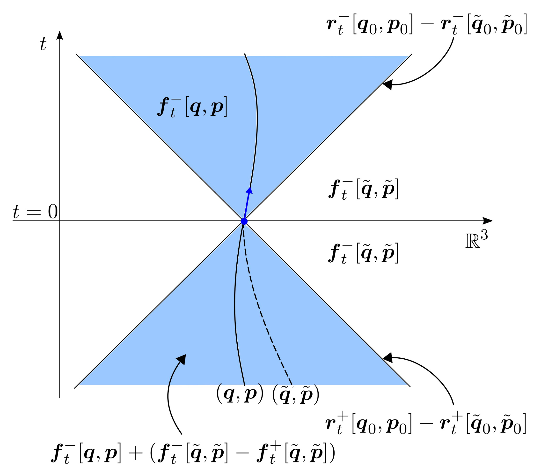
Figure: Support of the terms making up \(f_t\).

With the general solution formula \(\eqref{eq:f-general}\) we find an explanation for the emergence of the discussed singular light-front – homework.

The initial Coulomb field in \(\eqref{eq:ini-coulomb}\) read in terms of \(\eqref{eq:f-ini}\) for \(\lambda=1\) belongs to the Maxwell fields of an initially resting charge. In other words, the auxiliary trajectory \((\tilde{\vv q},\tilde{\vv p})\) fulfills \((\tilde{\vv q}^0,\tilde{\vv p}^0)=(\vv q^0,0)\) for all times \(t<0\). However, at initial time \(t=0\) the prescribe trajectory \((\vv q,\vv p)\) describes a charge with momentum \(\vv p^0\). Hence, the initial data we have prescribed in that example must physically be interpreted as an initial resting charge that at \(t=0\) suddenly accelerates instantly to acquire momentum \(\vv p^0\). This infinite acceleration causes the presence of the distributions in \(\eqref{eq:f-sol-coulomb-3}\).

Clearly, such solutions do not seem to make much sense and should therefore we eliminated. In order to do so, we must require another constraint in addition to the Maxwell constraint \(\eqref{eq:constraints-last}\):

• (C1): \(\tilde {\vv p}^0 = \vv p^0\).

In fact, \(f_t\) is a function on \(\bb R^3\setminus\{\vv q_t\}\) if and only if (C1) holds. Otherwise \(f_t\) will contain distributions with support of the boundary of the light-cone of \((\vv q^0,0)\) since the terms in \(\eqref{eq:f-boundary}\) do not cancel. This is however not the end of the story. Taking a close look at \(\eqref{eq:f-general}\) also reveals that unless

• (C2): \(\lim_{t\uparrow 0}\frac{d}{dt}\vv(\tilde {\vv p}_t) = \frac{d}{dt}\lim_{t\downarrow 0}\vv v(\vv p_t)\).

holds, the solution \(f_t\) is not a continuous function on \(\bb R^3\setminus\{\vv q_t\}\) because there is a step-discontinuity on the boundary of the light-cone of \((\vv q^0,0)\); which we shall call “shock light-front”.

The latter can be seen best when recasting \(\eqref{eq:f-general}\) into \[ \begin{align} \vv f_t = & 1_{B_{|t|}(\vv q_0)}\left(\vv f_t^{-\sigma(t)}[\vv q, \vv p] -\vv f_t^{-\sigma(t)}[\tilde{\vv q}, \tilde{\vv p}] \right) \label{eq:short-new} \\ & + \lambda \vv f_t^{-}[\tilde{\vv q}, \tilde{\vv p}] + (1- \lambda) \vv f_t^{+}[\tilde{\vv q}, \tilde{\vv p}] \label{eq:short-lw} \\ & + \vv r_t^{-\sigma(t)}[\vv q_0, \vv p_0]-\vv r_t^{-\sigma(t)}[\tilde{\vv q}_0, \tilde{\vv p}_0] \label{eq:short-dist} \\ & + \vv f_t^{0}. \label{eq:short-free} \end{align} \] Using the explicit formulas of the Liénard-Wiechert fields in \(\eqref{eq:lw}\) one finds that term \(\eqref{eq:short-new}\) only vanishes at the boundary of the light-cone of \((\vv q^0,0)\) if the condition (C2) is met. Hence, if conditions (C1) and (C2) hold, then we can read off the form \(\eqref{eq:f-general}\) that the only singularity lies at th position of the charge \(\vv q_t\) – recall Dirac’s computation that the terms \(f^-_t-f^+_t\) are not singular.

To conclude, in order to avoid the singular or shock-like light-fronts we have to impose a compatibility condition between the prescribed trajectory \(t\mapsto(\vv q_t,\vv p_t)\) and the initial fields \(f^0\). Not all prescribed charge trajectories and initial fields are admissible. As the initial fields \(f^0\) can always be expressed by means of \(\eqref{eq:f-ini}\) we may express this compatibility condition as one between the prescribed charge trajectory \(t\mapsto(\vv q_t,\vv p_t)\) and the auxiliary trajectory \(t\mapsto(\tilde{\vv q}_t,\tilde{\vv p}_t)\) in terms of (C1) and (C2). A violation of (C1) leads to singular light-fronts and a violation of (C2) to shock light-fronts.

5.4 Implications on the point-charge Maxwell-Lorentz system

Consider again the coupled system of Maxwell-Lorentz equations \(\eqref{eq:lorentz-point},\eqref{eq:maxwell-point},\eqref{eq:constraints-point}\) where the ill-defined self-interaction terms is omitted or replaced by an appropriately renormalized one. Ideally, we would expect to find a unique solution given the initial positions and momenta of the charges \(\vv q^0_i,\vv p^0_i\) and the initial electric and magnetic fields \(f^0_i=(\vv e^0_i,\vv b^0_i)\) for \(i=1,\ldots,N\). In light of the observation above, the immediate question is which of these initial data leads to singular or shock light-fronts.

Clearly, given the initial momentum \(\vv p_i^0\) of the charge \(i\) we may only allow initial fields \(f_i^0\) of the form \(\eqref{eq:f-ini}\) for an auxiliary trajectory \((\tilde{\vv q}_i,\tilde{\vv p}_i)\) fulfilling (C1), i.e., \(\tilde{\vv p}_i^0=\vv p_i^0\), to avoid singular light-fronts. As discussed above, should we fail to obey (C1) for \(i=1\), another charge, say \(i=2\), is bound to traverse the singular light-front and the dynamics breaks down at the moment of traversal.

Even when (C1) is fulfilled, (C2) might not and a shock light-front may develop. Every time the charges traverse such fronts it will cause their acceleration to jump spontaneously – a clearly unphysical behavior that should be avoided when computing solutions. However, this time we cannot simply assume that we pick initial data that obeys (C2). Recall that in order to check (C2) we need to know \[ \lim_{t\downarrow 0} \frac{d}{dt}\vv (\vv p_t), \] and hence, the acceleration is a positive neighborhood of \(t=0\). This data is, however, unknown unless we compute a solution. This poses the question whether the dynamics of the coupled Maxwell-Lorentz system for point-charges allows for an initial value problem formulation at all.

[homework]

References

Bauer, Gernot, and Detlef Dürr. 2001. “The Maxwell-Lorentz System of a Rigid Charge.” Annales Henri Poincaré 2 (1): 179–96. doi:10.1007/PL00001030.
Bauer, Gernot, Dirk - André Deckert Deckert, and Detlef Dürr. 2013. “Maxwell-Lorentz Dynamics of Rigid Charges.” Communications in Partial Differential Equations 38 (9): 1519–38. doi:10.1080/03605302.2013.814142.
Deckert, Dirk - André, and Vera Hartenstein. 2016. “On the Initial Value Formulation of Classical Electrodynamics.” ArXiv:1602.04685 [Math-Ph], February. http://arxiv.org/abs/1602.04685.
Dirac, Paul Adrien Maurice. 1938. “Classical Theory of Radiating Electrons.” Proceedings of the Royal Society of London A: Mathematical, Physical and Engineering Sciences 167 (929): 148–69. doi:10.1098/rspa.1938.0124.
Komech, Alexander, and Herbert Spohn. 2000. “Long—time Asymptotics for the Coupled Maxwell—Lorentz Equations.” Communications in Partial Differential Equations 25 (3-4): 559–84. doi:10.1080/03605300008821524.
Reed, Michael, and Barry Simon. 1975. Fourier Analysis, Self-Adjointness (Methods of Modern Mathematical Physics, Vol. 2). 1st ed. Academic Press.
Spohn, Herbert. 2008. Dynamics of Charged Particles and Their Radiation Field. 1 edition. Cambridge: Cambridge University Press.
Wheeler, John Archibald, and Richard Phillips Feynman. 1945. “Interaction with the Absorber as the Mechanism of Radiation.” Reviews of Modern Physics 17 (2-3): 157–81. doi:10.1103/RevModPhys.17.157.
———. 1949. “Classical Electrodynamics in Terms of Direct Interparticle Action.” Reviews of Modern Physics 21 (3): 425–33. doi:10.1103/RevModPhys.21.425.